The relation between Pearson’s correlation coefficient r and Salton’s cosine measure
Journal of the American Society for Information Science & Technology (forthcoming)
Leo Egghe 1,2 and Loet Leydesdorff 3
1. Universiteit Hasselt (UHasselt), Campus Diepenbeek, Agoralaan, B-3590 Diepenbeek, Belgium;[1] leo.egghe@uhasselt.be
2. Universiteit Antwerpen (UA), IBW, Stadscampus, Venusstraat 35, B-2000 Antwerpen, Belgium.
3. University of Amsterdam, Amsterdam School of Communication Research (ASCoR), Kloveniersburgwal 48, 1012 CX Amsterdam, The Netherlands; loet@leydesdorff.net
ABSTRACT
The relation
between Pearson’s correlation coefficient and Salton’s cosine measure is revealed
based on the different possible values of the division of the ![]() -norm and the
-norm and the ![]() -norm of a
vector. These different values yield a sheaf of increasingly straight lines
which form together a cloud of points, being the investigated relation. The
theoretical results are tested against the author co-citation relations among
24 informetricians for whom two matrices can be constructed, based on
co-citations: the asymmetric occurrence matrix and the symmetric co-citation
matrix. Both examples completely confirm the theoretical results. The results
enable us to specify an algorithm which provides a threshold value for the
cosine above which none of the corresponding Pearson correlations would be
negative. Using this threshold value can be expected to optimize the
visualization of the vector space.
-norm of a
vector. These different values yield a sheaf of increasingly straight lines
which form together a cloud of points, being the investigated relation. The
theoretical results are tested against the author co-citation relations among
24 informetricians for whom two matrices can be constructed, based on
co-citations: the asymmetric occurrence matrix and the symmetric co-citation
matrix. Both examples completely confirm the theoretical results. The results
enable us to specify an algorithm which provides a threshold value for the
cosine above which none of the corresponding Pearson correlations would be
negative. Using this threshold value can be expected to optimize the
visualization of the vector space.
Keywords: Pearson, correlation coefficient, Salton, cosine, non-functional relation, threshold
1. Introduction
Ahlgren, Jarneving & Rousseau (2003) questioned the use of Pearson’s correlation coefficient as a similarity measure in Author Cocitation Analysis (ACA) on the grounds that this measure is sensitive to zeros. Analytically, the addition of zeros to two variables should add to their similarity, but these authors demonstrated with empirical examples that this addition can depress the correlation coefficient between variables. Salton’s cosine is suggested as a possible alternative because this similarity measure is insensitive to the addition of zeros (Salton & McGill, 1983). In general, the Pearson coefficient only measures the degree of a linear dependency. One can expect statistical correlation to be different from the one suggested by Pearson coefficients if a relationship is nonlinear (Frandsen, 2004). However, the cosine does not offer a statistics.
In a reaction White (2003) defended the use of the Pearson correlation hitherto in ACA with the pragmatic argument that the differences resulting from the use of different similarity measures can be neglected in research practice. He illustrated this with dendrograms and mappings using Ahlgren, Jarneving & Rousseau’s (2003) own data. Leydesdorff & Zaal (1988) had already found marginal differences between results using these two criteria for the similarity. Bensman (2004) contributed a letter to the discussion in which he argued for the use of Pearson’s r for more fundamental reasons. Unlike the cosine, Pearson’s r is embedded in multivariate statistics, and because of the normalization implied, this measure allows for negative values.
Jones & Furnas (1987) explained the difference between Salton’s cosine and Pearson’s correlation coefficient in geometrical terms, and compared both measures with a number of other similarity criteria (Jaccard, Dice, etc.). The Pearson correlation normalizes the values of the vectors to their arithmetic mean. In geometrical terms, this means that the origin of the vector space is located in the middle of the set, while the cosine constructs the vector space from an origin where all vectors have a value of zero (Figure 1).
|
|
|
|
|
|
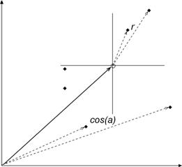
Figure 1: The difference between Pearson’s r and Salton’s cosine is geometrically equivalent to a translation of the origin to the arithmetic mean values of the vectors.
Consequently, the Pearson correlation can vary from –1 to + 1,[2] while the cosine varies only from zero to one in a single quadrant. In the visualization—using methods based on energy optimization of a system of springs (Kamada & Kawai, 1989) or multidimensional scaling (MDS; see: Kruskal & Wish, 1973; Brandes & Pich, 2007)—this variation in the Pearson correlation is convenient because one can distinguish between positive and negative correlations. Leydesdorff (1986; cf. Leydesdorff & Cozzens, 1993), for example, used this technique to illustrate factor-analytical results of aggregated journal-journal citations matrices with MDS-based journal maps.
Although in many practical cases, the differences between using Pearson’s correlation coefficient and Salton’s cosine may be negligible, one cannot estimate the significance of this difference in advance. Given the fundamental nature of Ahlgren, Jarneving & Rousseau’s (2003, 2004) critique, in our opinion, the cosine is preferable for the analysis and visualization of similarities. Of course, a visualization can be further informed on the basis of multivariate statistics which may very well have to begin with the construction of a Pearson correlation matrix (as in the case of factor analysis). In practice, therefore, one would like to have theoretically informed guidance about choosing the threshold value for the cosine values to be included or not. However, because of the different metrics involved there is no one-to-one correspondence between a cut-off level of r = 0 and a value of the cosine similarity.
Since negative correlations also lead to positive cosine values, the cut-off level is no longer given naturally in the case of the cosine, and, therefore, the choice of a threshold remains somewhat arbitrary (Leydesdorff, 2007a). Yet, variation of the threshold can lead to different visualizations (Leydesdorff & Hellsten, 2006). Using common practice in social network analysis, one could consider using the mean of the lower triangle of the similarity matrix as a threshold for the display (Wasserman & Faust, 1994, at pp. 407f.), but this solution often fails to satisfy the criterion of generating correspondence between, for example, the factor-analytically informed clustering and the clusters visible on the screen.
Ahlgren, Jarneving & Rousseau (2003 at p. 554) downloaded from the Web of Science 430 bibliographic descriptions of articles published in Scientometrics and 483 such descriptions published in the Journal of the American Society for Information Science and Technology (JASIST) for the period 1996-2000. From the 913 bibliographic references in these articles they composed a co-citation matrix for 12 authors in the field of information retrieval and 12 authors doing bibliometric-scientometric research. They provide both the co-occurrence matrix and the Pearson correlation table in their paper (at p. 555 and 556, respectively).
Leydesdorff & Vaughan (2006) repeated the analysis in order to obtain the original (asymmetrical) data matrix. Using precisely the same searches, these authors found 469 articles in Scientometrics and 494 in JASIST on 18 November 2004. The somewhat higher numbers are consistent with the practice of Thomson Scientific (ISI) to reallocate papers sometimes at a later date to a previous year. Thus, these differences can be disregarded.
First, we will use the asymmetric occurrence data containing only 0s and 1s: 279 papers contained at least one co-citation to two or more authors on the list of 24 authors under study (Leydesdorff & Vaughan, 2006, p.1620). In this case of an asymmetrical occurrence matrix, an author receives a 1 on a coordinate (representing one of these papers) if he /she is cited in this paper and a score 0 if not. This table is not included here or in Leydesdorff (2008) since it is long (but it can be obtained from the authors upon request).
As a second example, we use the
symmetric co-citation data as provided by Leydesdorff (2008, p. 78), Table 1
(as described above). On the basis of this data, Leydesdorff (2008, at p. 78)
added the values on the main diagonal to Ahlgren, Jarneving & Rousseau’s
(2003) Table 7 which provided the author co-citation data (p. 555). The data
allows us to compare the various similarity matrices using both the symmetrical
co-occurrence data and the asymmetrical occurrence data (Leydesdorff &
Vaughan, 2006; Waltman & van Eck, 2007; Leydesdorff, 2007b). This data will
be further analyzed after we have established our mathematical model on the
relation between Pearson’s correlation coefficient r and Salton’s cosine
measure![]() .
.
3. Formalization of the problem
In a recent contribution, Leydesdorff (2008) suggested that in the case of a symmetrical co-occurrence matrix, Small’s (1973) proposal to normalize co-citation data using the Jaccard index (Jaccard, 1901; Tanimoto, 1957) has conceptual advantages over the use of the cosine. On the basis of Figure 3 of Leydesdorff (2008, at p. 82), Egghe (2008) was able to show using the same data that all these similarity criteria can functionally be related to one another. The results in Egghe (2008) can be outlined as follows.
Let ![]() and
and ![]() be two vectors
where all the coordinates are positive. The Jaccard index of these two vectors
(measuring the “similarity” of these vectors) is defined as
be two vectors
where all the coordinates are positive. The Jaccard index of these two vectors
(measuring the “similarity” of these vectors) is defined as
 (1)
(1)
 (2)
(2)
where ![]() is the inproduct of the
vectors
is the inproduct of the
vectors ![]() and
and
![]() and
where
and
where  and
and
 are
the Euclidean norms of
are
the Euclidean norms of ![]() and
and ![]() (also called the
(also called the ![]() -norms).
Salton’s cosine measure is defined as
-norms).
Salton’s cosine measure is defined as
 (3)
(3)
 (4)
(4)
in the same notation as above.
Among other results we could prove that, if ![]() , then
, then
![]() (5)
(5)
a simple relation, agreeing completely with the experimental findings.
For Dice’s measure E:
 (6)
(6)
 (7)
(7)
we could even prove that, if ![]() , we have
, we have ![]() . The same
could be shown for several other similarity measures (Egghe, 2008). We refer
the reader to some classical monographs which define and apply several of these
measures in information science: Boyce, Meadow & Kraft (1995);
Tague-Sutcliffe (1995); Grossman & Frieder (1998); Losee (1998); Salton
& McGill (1987) and Van Rijsbergen (1979); see also Egghe & Michel
(2002, 2003).
. The same
could be shown for several other similarity measures (Egghe, 2008). We refer
the reader to some classical monographs which define and apply several of these
measures in information science: Boyce, Meadow & Kraft (1995);
Tague-Sutcliffe (1995); Grossman & Frieder (1998); Losee (1998); Salton
& McGill (1987) and Van Rijsbergen (1979); see also Egghe & Michel
(2002, 2003).
Egghe (2008) mentioned the problem of relating Pearson’s correlation coefficient with the other measures. The definition of r is:
 (8)
(8)
In this study, we address this remaining question about the relation between Pearson’s correlation coefficient and Salton’s cosine.
The problem lies in the
simultaneous occurrence of the ![]() -norms of the vectors
-norms of the vectors ![]() and
and ![]() and the
and the ![]() -norms of
these vectors in the definition of the Pearson correlation coefficient. The
-norms of
these vectors in the definition of the Pearson correlation coefficient. The ![]() -norms are
defined as follows:
-norms are
defined as follows:
![]() (9)
(9)
![]() (10)
(10)
These ![]() -norms are the basis for the
so-called “city-block metric” (cf. Egghe & Rousseau, 1990). The
-norms are the basis for the
so-called “city-block metric” (cf. Egghe & Rousseau, 1990). The ![]() -norms were
not occurring in the other measures defined above, and therefore not in Egghe
(2008). This makes r a special measure in this context. In Ahlgren,
Jarneving & Rousseau (2003) argued that r lacks some properties that
similarity measures should have. Of course, Pearson’s r remains a very
important measure of the degree to which a regression line fits an experimental
two-dimensional cloud of points. (See Egghe & Rousseau (2001) for many
examples in library and information science.)
-norms were
not occurring in the other measures defined above, and therefore not in Egghe
(2008). This makes r a special measure in this context. In Ahlgren,
Jarneving & Rousseau (2003) argued that r lacks some properties that
similarity measures should have. Of course, Pearson’s r remains a very
important measure of the degree to which a regression line fits an experimental
two-dimensional cloud of points. (See Egghe & Rousseau (2001) for many
examples in library and information science.)
Basic for determining the relation
between r and ![]() will be, evidently, the relation
between the
will be, evidently, the relation
between the ![]() -
and the
-
and the ![]() -norms
of the vectors
-norms
of the vectors ![]() and
and ![]() . In the next section we show
that every fixed value of
. In the next section we show
that every fixed value of  and of
  yields a linear relation
between r and
yields a linear relation
between r and ![]() .
.
4. The mathematical model for the relation between r and Cos
Let ![]() and
and ![]() the two
vectors of length
the two
vectors of length ![]() . Denote
. Denote
(11)
and
(12)
(notation as in
the previous section). Note that, trivially, ![]() and
and ![]() . We also have that
. We also have that ![]() and
and ![]() . Indeed, by
the inequality of Cauchy-Schwarz (e.g. Hardy, Littlewood & Pólya, 1988) we
have
. Indeed, by
the inequality of Cauchy-Schwarz (e.g. Hardy, Littlewood & Pólya, 1988) we
have
![]()
Hence

But, if we suppose
that ![]() is
not the constant vector, we have that
is
not the constant vector, we have that ![]() , hence, by the above,
, hence, by the above, ![]() . The same argument
goes for
. The same argument
goes for ![]() ,
yielding
,
yielding ![]() .
We have the following result.
.
We have the following result.
Proposition II.1:
The following
relation is generally valid, given (11) and (12) and if ![]() nor
nor ![]() are
constant vectors
are
constant vectors
![]() (13)
(13)
Note that, by the
above, the numbers under the roots are positive (and strictly positive neither ![]() nor
nor ![]() is
constant).
is
constant).
Proof:
Define the “Pseudo
Cosine” measure ![]()
 (14)
(14)
One can find
earlier definitions in Jones & Furnas (1987). The measure is called “Pseudo
Cosine” since, in formula (3) (the real Cosine of the angle between the vectors
![]() and
and
![]() ,
which is well-known), one replaces
,
which is well-known), one replaces ![]() and
and ![]() by
by ![]() and
and ![]() ,
respectively. Hence, as follows from (4) and (14) we have
,
respectively. Hence, as follows from (4) and (14) we have
 ,
(15)
,
(15)
using (11) and
(12). Now we have, since neither ![]() nor
nor ![]() is constant (avoiding
is constant (avoiding ![]() in the
next expression).
in the
next expression).
by (11), (12) and (14). By (15) we now have
from which ![]() can be
resolved:
can be
resolved:
![]() (16)
(16)
Since we want the inverse of (16) we have, from (16), that (13) is correct.
Note that (13) is a linear relation
between r and ![]() , but dependent on the parameters
, but dependent on the parameters ![]() and
and ![]() (note
that
(note
that ![]() is
constant, being the length of the vectors
is
constant, being the length of the vectors ![]() and
and ![]() ).
).
Note that ![]() if and only if
if and only if
![]() (17)
(17)
and that r = 0 if and only if
![]() (18)
(18)
Both formulae vary with variable ![]() and
and ![]() , but (17) is
always negative and (18) is always positive. Hence, for varying
, but (17) is
always negative and (18) is always positive. Hence, for varying ![]() and
and ![]() , we have
obtained a sheaf of increasingly straight lines. Since, in practice,
, we have
obtained a sheaf of increasingly straight lines. Since, in practice, ![]() and
and ![]() will
certainly vary (i.e. the numbers
will
certainly vary (i.e. the numbers ![]() will not be the same for all
vectors) we have proved here that the relation between r and
will not be the same for all
vectors) we have proved here that the relation between r and ![]() is not a
functional relation (as was the case between all other measures, as discussed
in the previous section) but a relation as an increasing cloud of points.
Furthermore, one can expect the cloud of points to occupy a range of points,
for
is not a
functional relation (as was the case between all other measures, as discussed
in the previous section) but a relation as an increasing cloud of points.
Furthermore, one can expect the cloud of points to occupy a range of points,
for ![]() ,
below the zero ordinate while, for r = 0, the cloud of points will
occupy a range of points with positive abscissa values (this is obvious since
,
below the zero ordinate while, for r = 0, the cloud of points will
occupy a range of points with positive abscissa values (this is obvious since ![]() while
all vector coordinates are positive). Note also that (17) (its absolute value)
and (18) decrease with
while
all vector coordinates are positive). Note also that (17) (its absolute value)
and (18) decrease with ![]() , the length of the vector (for fixed
, the length of the vector (for fixed ![]() and
and ![]() ). This is
also the case for the slope of (13), going, for large
). This is
also the case for the slope of (13), going, for large ![]() , to 1, as is readily
seen (for fixed
, to 1, as is readily
seen (for fixed ![]() and
and ![]() ).
).
All these findings will be confirmed in the next section where exact numbers will be calculated and compared with the experimental graphs.
5. One example and two applications
As noted, we re-use the reconstructed data set of Ahlgren, Jarneving & Rousseau (2003) which was also used in Leydesdorff (2008). This data deals with the co-citation features of 24 informetricians. We distinguish two types of matrices (yielding the different vectors representing the 24 authors).
First, we use the
binary asymmetric occurrence matrix: a matrix of size 279 x 24 as described in
section 2. Then, we use the symmetric co-citation matrix of size 24 x 24 where
the main diagonal gives the number of papers in which an author is cited – see
Table 1 in Leydesdorff (2008, at p. 78). Although these matrices are
constructed from the same data set, it will be clear that the corresponding
vectors are very different: in the first case all vectors have binary values and
length ![]() ;
in the second case the vectors are not binary and have length
;
in the second case the vectors are not binary and have length ![]() . So these two
examples will also reveal the n-dependence of our model, as described above.
. So these two
examples will also reveal the n-dependence of our model, as described above.
5.1 The case of the binary asymmetric occurrence matrix
Here ![]() . Hence the
model (13) (and its consequences such as (17) and (18)) are known as soon as we
have the values
. Hence the
model (13) (and its consequences such as (17) and (18)) are known as soon as we
have the values ![]() and
and ![]() as in (11) and (12), i.e.,
we have to know the values
as in (11) and (12), i.e.,
we have to know the values ![]() for every author, represented by
for every author, represented by ![]() . Since all
vectors are binary we have, for every vector
. Since all
vectors are binary we have, for every vector ![]() :
:
 (19)
(19)
We have the data as in Table 1. They are nothing other than the square roots of the main diagonal elements in Table 1 in Leydesdorff (2008).
Table
1. ![]() for
the 24 authors
for
the 24 authors
|
Author |
|
|
Braun |
|
|
Schubert |
|
|
Glänzel |
|
|
Moed |
|
|
Nederhof |
|
|
Narin |
|
|
Tyssen |
|
|
van Raan |
|
|
Leydesdorff |
|
|
Price |
|
|
Callon |
|
|
Cronin |
|
|
Cooper |
|
|
Van Rijsbergen |
|
|
Croft |
|
|
Robertson |
|
|
Blair |
|
|
Harman |
|
|
Belkin |
|
|
Spink |
|
|
Fidel |
|
|
Marchionini |
|
|
Kuhltau |
|
|
Dervin |
|
For (13) we do not
need the a- and ![]() -values of all authors: to see the range
of the
-values of all authors: to see the range
of the ![]() -values,
given a
-values,
given a ![]() -value
we only calculate (13) for the two smallest and largest values for
-value
we only calculate (13) for the two smallest and largest values for ![]() and
and ![]() .
.
1. Smallest values: ![]() ,
, ![]()
yielding ![]()
2. Largest values: ![]() ,
, ![]()
yielding ![]()
This is a rather
rough argument: not all a- and b-values occur at every fixed ![]() -value so that
better approximations are possible, but for the sake of simplicity we will use
the larger margins above: if we can approximate the experimental graphical
relation between
-value so that
better approximations are possible, but for the sake of simplicity we will use
the larger margins above: if we can approximate the experimental graphical
relation between ![]() and
and ![]() in a satisfactory way, the
model is approved.
in a satisfactory way, the
model is approved.
Using (13), (17)
or (18) we obtain, in each case, the range in which we expect the practical (![]() ) points to
occur. For
) points to
occur. For ![]() we
have r between
we
have r between ![]() and
and ![]() (by (17)). For
(by (17)). For ![]() we have
by (18),
we have
by (18), ![]() between
between
![]() and
and
![]() .
Further, by (13), for
.
Further, by (13), for ![]() we have r between
we have r between ![]() and
and ![]() . For
. For ![]() we have r
between
we have r
between ![]() and
and
![]() .
For
.
For ![]() we
have r between
we
have r between ![]() and
and ![]() . Finally for
. Finally for ![]() we have r
between
we have r
between ![]() and
and
![]() and
for
and
for ![]() we
have r between
we
have r between ![]() and
and ![]() . We do not go further due to
the scarcity of the data points.
. We do not go further due to
the scarcity of the data points.
The experimental (![]() ) cloud of
points and the limiting ranges of the model are shown together in Fig. 2, so
that the comparison is easy.
) cloud of
points and the limiting ranges of the model are shown together in Fig. 2, so
that the comparison is easy.
|
|
|
|
|
|
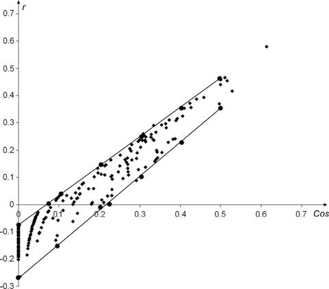
Figure 2: Data points (![]() ) for the binary asymmetric occurrence
matrix and ranges of the model.
) for the binary asymmetric occurrence
matrix and ranges of the model.
For reasons of
visualization we have connected the calculated ranges. Figure 2 speaks for
itself. The indicated straight lines are the upper and lower lines of the sheaf
of straight lines composing the cloud of points. The higher the straight line,
the smaller its slope. The r-range (thickness) of the cloud decreases as
![]() increases.
We also see that the negative r-values, e.g. at
increases.
We also see that the negative r-values, e.g. at ![]() , are explained,
although the lowest fitted point on
, are explained,
although the lowest fitted point on ![]() is a bit too low due to the fact
that we use the total
is a bit too low due to the fact
that we use the total ![]() range while, on
range while, on ![]() , not
all a- and b-values occur.
, not
all a- and b-values occur.
We can
say that the model (13) explains the obtained (![]() ) cloud of points.
We will now do the same for the other matrix. We will then be able to compare
both clouds of points and both models.
) cloud of points.
We will now do the same for the other matrix. We will then be able to compare
both clouds of points and both models.
5.2 The case of the symmetric co-citation matrix
Here ![]() . Based on
Table 1 in Leydesdorff (2008), we have the values of
. Based on
Table 1 in Leydesdorff (2008), we have the values of ![]() . For example, for
“Braun” in the first column of this table,
. For example, for
“Braun” in the first column of this table, ![]() and
and  . In this case,
  . The values
of
. The values
of ![]() for
all 24 authors, represented by their respective vector
for
all 24 authors, represented by their respective vector ![]() , are provided in Table
2.
, are provided in Table
2.
Table
2: ![]() for
the 24 authors
for
the 24 authors
|
Author |
|
|
Braun |
2.5032838 |
|
Schubert |
2.4795703 |
|
Glänzel |
2.729457 |
|
Moed |
2.7337391 |
|
Nederhof |
2.8221626 |
|
Narin |
2.8986697 |
|
Tyssen |
3.0789273 |
|
van Raan |
2.4077981 |
|
Leydesdorff |
2.8747094 |
|
Price |
2.7635278 |
|
Callon |
2.8295923 |
|
Cronin |
2.556743 |
|
Cooper |
2.3184046 |
|
Van Rijsbergen |
2.4469432 |
|
Croft |
3.0858543 |
|
Robertson |
2.920658 |
|
Blair |
2.517544 |
|
Harman |
2.5919129 |
|
Belkin |
2.8555919 |
|
Spink |
3.0331502 |
|
Fidel |
2.6927563 |
|
Marchionini |
2.4845716 |
|
Kuhltau |
2.4693658 |
|
Dervin |
2.5086617 |
As in the previous
example, we only use the two smallest and largest values for ![]() and
and ![]() .
.
1. Smallest values: ![]() ,
, ![]()
yielding ![]()
2. Largest values: ![]() ,
, ![]()
yielding ![]()
As in the first
example, the obtained ranges will probably be a bit too large, since not all a-
and b-values occur at every ![]() -value. We will now investigate the
quality of the model in this case.
-value. We will now investigate the
quality of the model in this case.
If ![]() then, by
(17) we have that r is between
then, by
(17) we have that r is between ![]() and
and ![]() . If r = 0 we have that
. If r = 0 we have that ![]() is
between
is
between ![]() and
and
![]() ,
using (18). For
,
using (18). For ![]() we have that r is between
we have that r is between ![]() and
and ![]() . For
. For ![]() , r is
between
, r is
between ![]() and
and
![]() .
. ![]() implies
that r is between
implies
that r is between ![]() and
and ![]() .
. ![]() implies that r is
between
implies that r is
between ![]() and
and
![]() and
finally, for
and
finally, for ![]() we have that r is between
we have that r is between ![]() and
and ![]() .
.
The experimental ![]() cloud of points and the limiting
ranges of the model in this case are shown together in Figure 3.
cloud of points and the limiting
ranges of the model in this case are shown together in Figure 3.
|
|
|
|
|
|
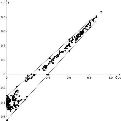
Figure 3: Data points ![]() for the symmetric co-citation matrix and ranges of
the model.
for the symmetric co-citation matrix and ranges of
the model.
The same
properties are found here as in the previous case, although the data are
completely different. Again the lower and upper straight lines, delimiting the cloud
of points, are clear. They also delimit the sheaf of straight lines, given by
(13). Again, the higher the straight line, the smaller its slope. The r-range
(thickness) of the cloud decreases as ![]() increases. This effect is stronger
in Fig. 3 than in Fig. 2. We again see that the negative values of r,
e.g. at
increases. This effect is stronger
in Fig. 3 than in Fig. 2. We again see that the negative values of r,
e.g. at ![]() ,
are explained.
,
are explained.
We conclude that
the model (13) explains the obtained ![]() cloud of points.
cloud of points.
6. The effects of the predicted threshold values on the visualization
Figure 4 provides a visualization using the asymmetrical matrix (n = 279) and the Pearson correlation for the normalization.[3] Negative values for the Pearson correlation are indicated with dashed edges.
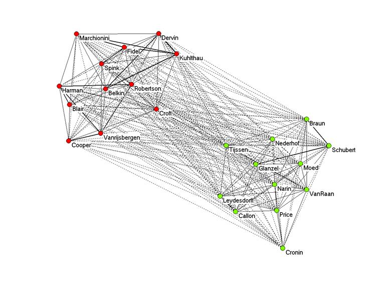
Figure 4: Pearson correlation among citation patterns of 24 authors in the information sciences in 279 citing documents.
Only positive correlations are indicated within each of the two groups with the single exception of a correlation (r = 0.031) between the citation patterns of “Croft” and “Tijssen.” This r = 0.031 accords with cosine = 0.101. In section 5.1, it was shown that given this matrix (n = 279), r = 0 ranges for the cosine between 0.068 and 0.222. Figure 2 (above) showed that several points are within this range. However, there are also negative values for r within each of the two main groups. For example, “Cronin” has positive correlations with only five of the twelve authors in the group on the lower right side: “Narin” (r = 0.11), “Van Raan” (r = 0.06), “Leydesdorff” (r = 0.21), “Callon” (r = 0.08), and “Price” (r = 0.14). All other correlations of “Cronin” are negative.
If we use the lower limit for the threshold value of the cosine (0.068), we obtain Figure 5.
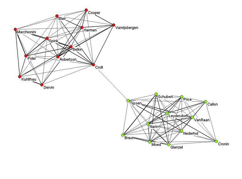
Figure 5: Visualization of the same matrix based on cosine > 0.068.
The two groups are now separated, but connected by the one positive correlation between “Tijssen” and “Croft”. This is fortunate because this correlation is above the threshold value. In addition to relations to the five author names correlated positively to “Cronin”, however, “Cronin” is in this representation erroneously connected to “Moed” (r = − 0.02), “Nederhof” (r = − 0.03), and “Glanzel” (r = − 0.05).
Figure 6 provides the visualization using the upper limit of the threshold value (0.222).
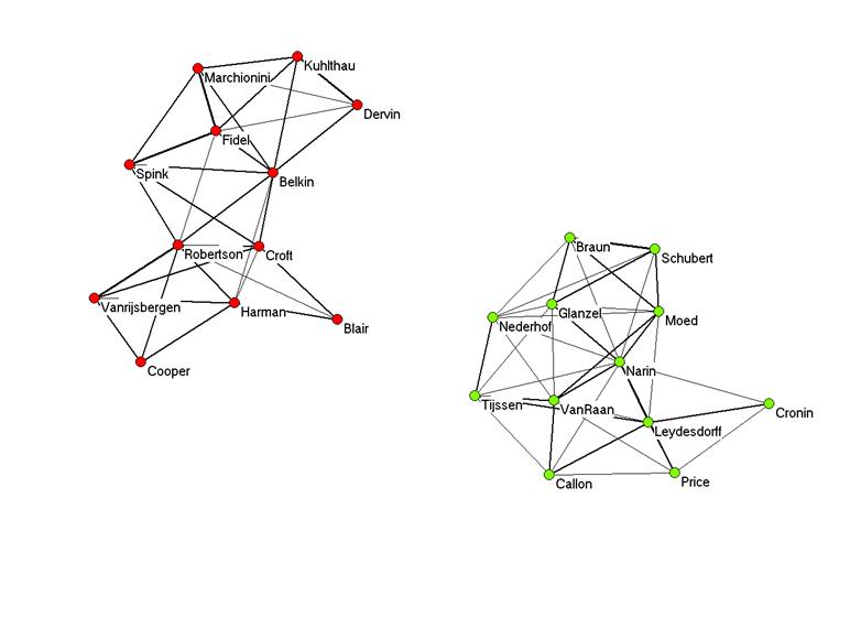
Figure 6: Visualization of the same matrix based on cosine > 0.222.
In this visualization, the two groups are no longer connected, and thus the correlation between “Croft” and “Tijssen” (r = 0.31) is not appreciated. Similarly, the correlation of “Cronin” with two other authors at a level of r < 0.1 (“Van Raan” and “Callon”) is no longer visualized. However, all correlations at the level of r > 0.1 are made visible. (Since these two graphs are independent, the optimization using Kamada & Kawai’s (1989) algorithm was repeated.) The graphs are additionally informative about the internal structures of these communities of authors. Using this upper limit of the threshold value, in summary, prevents the drawing of edges which correspond with negative correlations, but is conservative. This is a property which one would like in most representations.
|
|
|
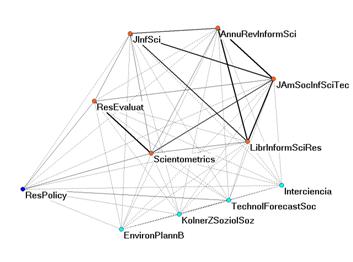
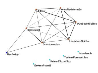
Figure 7a and b: Eleven journals in the citation impact environment of Scientometrics in 2007 with and without negative correlations in citation patterns.
Figure 7 shows the use of the upper limit of the threshold value for the cosine (according with r = 0) in another application. On the left side (Figure 7a), the citation impact environment (“cited patterns”) of the eleven journals which cited Scientometrics in 2007 to the extent of more than 1% of its total number of citations in this year (n = 1515) is visualized using the Pearson correlation coefficients among the citation patterns. Negative values of r are depicted as dashed lines.
The right-hand figure can be generated by deleting these dashed edges. However, this Figure 7b is based on using the upper limit of the cosine for r = 0, that is, cosine > 0.301. The use of the cosine enhances the edges between the journal Research Policy, on the one hand, and Research Evaluation and Scientometrics, on the other. These relations were depressed because of the zeros prevailing in the comparison with other journals in this set (Ahlgren et al., 2003). Thus, the use of the cosine improves on the visualizations, and the cosine value predicted by the model provides us with a useful threshold.
In summary, the use of the upper limit of the cosine which corresponds to the value of r = 0 can be considered conservative, but warrants focusing on the meaningful part of the network when using the cosine as similarity criterion. In the meantime, this “Egghe-Leydesdorff” threshold has been implemented in the output of the various bibliometric programs available at http://www.leydesdorff.net/software.htm for users who wish to visualize the resulting cosine-normalized matrices.
7. The relation between r and similarity measures other than Cos
In the
introduction we noted the functional relationships between ![]() and other
similarity measures such as Jaccard, Dice, etc. Based on
and other
similarity measures such as Jaccard, Dice, etc. Based on ![]() -norm relations, e.g.
-norm relations, e.g. ![]() (but
generalizations are given in Egghe (2008)) we could prove in Egghe (2008) that
(
(but
generalizations are given in Egghe (2008)) we could prove in Egghe (2008) that
(![]() =
Jaccard)
=
Jaccard)
![]() (20)
(20)
and that ![]() (
(![]() = Dice), and
the same holds for the other similarity measures discussed in Egghe (2008). It
is then clear that the combination of these results with (13) yields the
relations between r and these other measures. Under the above
assumptions of
= Dice), and
the same holds for the other similarity measures discussed in Egghe (2008). It
is then clear that the combination of these results with (13) yields the
relations between r and these other measures. Under the above
assumptions of ![]() -norm equality we see, since
-norm equality we see, since ![]() , that (13) is
also valid for
, that (13) is
also valid for ![]() replaced by
replaced by ![]() . For
. For ![]() , using (13)
and (20) one obtains:
, using (13)
and (20) one obtains:
![]() (21)
(21)
and hence
![]() (22)
(22)
which is a relation as depicted in Figure 8, for the first example (the asymmetric binary occurrence matrix case).
|
|
|
|
|
|
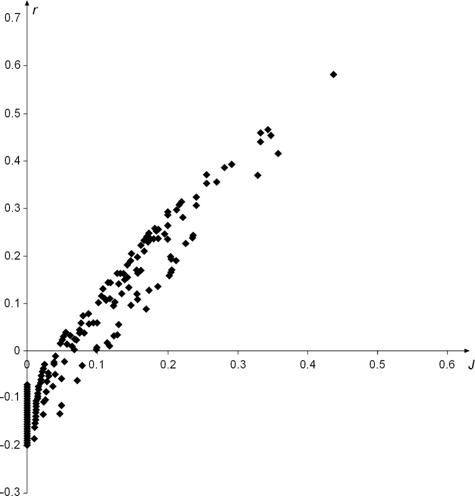
Figure 8: The relation between r and J for the binary asymmetric occurrence matrix
The faster increase
of this cloud of points, compared with the one in Figure 2 follows from the
fact that (20) implies that ![]() (since
(since ![]() ) if
) if ![]() : in fact
: in fact ![]() is
convexly increasing in
is
convexly increasing in ![]() , below the first bissectrix: see
Leydesdorff (2008) and Egghe (2008).
, below the first bissectrix: see
Leydesdorff (2008) and Egghe (2008).
As we showed in
Egghe (2008), if ![]() all the other similarity measures
are equal to
all the other similarity measures
are equal to ![]() , so that we evidently have graphs as in
Figures 2 and 3 of the relation between r and the other measures.
, so that we evidently have graphs as in
Figures 2 and 3 of the relation between r and the other measures.
8. Conclusion
In this paper we
have presented a model for the relation between Pearson’s correlation
coefficient r and Salton’s cosine measure. We have shown that this relation
is not a pure function, but that the cloud of points ![]() can be described
by a sheaf of increasing straight lines whose slopes decrease, the higher the
straight line is in the sheaf. The negative part of r is explained, and
we have explained why the r-range (thickness) of the cloud decreases
when
can be described
by a sheaf of increasing straight lines whose slopes decrease, the higher the
straight line is in the sheaf. The negative part of r is explained, and
we have explained why the r-range (thickness) of the cloud decreases
when ![]() increases.
All these theoretical findings are confirmed on two data sets from Ahlgren,
Jarneving & Rousseau (2003) using co-citation data for 24 informetricians:
vectors in the asymmetric occurrence matrix and the symmetric co-citation
matrix.
increases.
All these theoretical findings are confirmed on two data sets from Ahlgren,
Jarneving & Rousseau (2003) using co-citation data for 24 informetricians:
vectors in the asymmetric occurrence matrix and the symmetric co-citation
matrix.
The algorithm enables
us to determine the threshold value for the cosine above which none of the
corresponding Pearson correlation coefficients on the basis of the same data
matrix will be lower than zero. In general, a cosine can never correspond with
an r < 0, if one divides the product between the two largest values
for a and b (that is,  for each vector) by the size of the
vector n.
for each vector) by the size of the
vector n.
In the case of Table 1, for example, the
two largest sumtotals in the asymmetrical matrix were 64 (for Narin) and 60
(for Schubert). Therefore, a was ![]() and b was
and b was ![]() and hence
and hence ![]() was
was ![]() . Since
. Since ![]() in this
case, the cosine should be chosen above 61.97/279 =
in this
case, the cosine should be chosen above 61.97/279 = ![]() because above
this threshold one expects no single Pearson correlation to be negative. This
cosine threshold value is sample (that is, n-) specific. However, one can
automate the calculation of this value for any dataset by using Equation 18.
because above
this threshold one expects no single Pearson correlation to be negative. This
cosine threshold value is sample (that is, n-) specific. However, one can
automate the calculation of this value for any dataset by using Equation 18.
References
P. Ahlgren, B. Jarneving and R. Rousseau (2003). Requirements for a cocitation similarity measure, with special reference to Pearson’s correlation coefficient. Journal of the American Society for Information Science and Technology 54(6), 550-560.
P. Ahlgren, B. Jarneving and R. Rousseau (2004). Autor cocitation and Pearson’s r. Journal of the American Society for Information Science and Technology 55(9), 843.
Bensman, S. J. (2004). Pearson’s r and Author Cocitation Analysis: A commentary on the controversy. Journal of the American Society for Information Science and Technology 55(10), 935-936.
Brandes, U., and Pich, C. (2007). Eigensolver Methods for Progressive Multidimensional Scaling of Large Data. In M. Kaufmann & D. Wagner (Eds.), Graph Drawing, Karlsruhe, Germany, September 18-20, 2006 (Lecture Notes in Computer Science, Vol. 4372, pp. 42-53). Berlin, Heidelberg: Springer.
B.R. Boyce, C.T. Meadow and D.H. Kraft (1995). Measurement in Information Science. Academic Press, New York, NY, USA.
L. Egghe (2008). New relations between similarity measures for vectors based on vector norms. Preprint.
L. Egghe and C. Michel (2002). Strong similarity measures for ordered sets of documents in information retrieval. Information Processing and Management 38(6), 823-848.
L. Egghe and C. Michel (2003). Construction of weak and strong similarity measures for ordered sets of documents using fuzzy set techniques. Information Processing and Management 39(5), 771-807.
L. Egghe and R. Rousseau (1990). Introduction to Informetrics. Quantitative Methods in Library, Documentation and Information Science. Elsevier, Amsterdam.
L. Egghe and R. Rousseeau (2001). Elementary Statistics for Effective Library and Information Service Management. Aslib imi, London, UK.
T. F. Frandsen (2004). Journal diffusion factors – a measure of diffusion ? Aslib Proceedings: new Information Perspectives 56(1), 5-11.
D.A. Grossman and O. Frieder (1998). Information Retrieval Algorithms and Heuristics. Kluwer Academic Publishers, Boston, MA, USA.
G. Hardy, J.E. Littlewood and G. Pólya (1988). Inequalities. Cambridge University Press, Cambridge, UK.
P. Jaccard (1901). Distribution de la flore alpine dans le Bassin des Drouces et dans quelques regions voisines. Bulletin de la Société Vaudoise des Sciences Naturelles 37(140), 241–272.
W. P. Jones and G. W. Furnas (1987). Pictures of relevance: a geometric analysis of similarity measures. Journal of the American Society for Information Science 36(6), 420-442.
Kamada, T., and Kawai, S. (1989). An algorithm for drawing general undirected graphs. Information Processing Letters, 31(1), 7-15.
Kruskal, J. B., and Wish, M. (1978). Multidimensional Scaling. Beverly Hills, CA: Sage Publications.
L. Leydesdorff (2007a). Visualization of the citation impact environments of scientific journals: an online mapping exercise. Journal of the American Society of Information Science and Technology 58(1), 207-222.
L. Leydesdorff (2007b). Should co-occurrence data be normalized ? A rejoinder. Journal of the American Society for Information Science and Technology 58(14), 2411-2413.
L. Leydesdorff (2008). On the normalization and visualization of author co-citation data: Salton’s cosine versus the Jaccard index. Journal of the American Society for Information Science and Technology 59(1), 77-85.
L. Leydesdorff and S.E. Cozzens (1993). The delineation of specialties in terms of journals using the dynamic journal set of the Science Citation Index. Scientometrics 26, 133-154.
L. Leydesdorff and I. Hellsten (2006). Measuring the meaning of words in contexts: an automated analysis of controversies about ‘Monarch butterflies,’ ‘Frankenfoods,’ and ‘stem cells’. Scientometrics 67(2), 231-258.
L. Leydesdorff and L. Vaughan (2006). Co-occurrence matrices and their applications in information science: extending ACA to the Web environment. Journal of the American Society for Information Science and Technology 57(12), 1616-1628.
L. Leydesdorff and R. Zaal (1988). Co-words and citations. Relations between document sets and environments. In L. Egghe and R. Rousseau (Eds.), Informetrics 87/88, 105-119, Elsevier, Amsterdam.
R.M. Losee (1998). Text Retrieval and Filtering: Analytical Models of Performance. Kluwer Academic Publishers, Boston, MA, USA.
G. Salton and M.J. McGill (1987). Introduction to Modern Information Retrieval. McGraw-Hill, New York, NY, USA.
H. Small (1973). Co-citation in the scientific literature: A new measure of the relationship between two documents. Journal of the American Society for Information Science 24(4), 265-269.
J. Tague-Sutcliffe (1995). Measuring Information: An Information Services Perspective. Academic Press, New York, NY, USA.
T. Tanimoto (1957). Internal report: IBM Technical Report Series, November, 1957.
C.J. Van Rijsbergen (1979). Information Retrieval. Butterworths, London, UK.
L. Waltman and N.J. van Eck (2007). Some comments on the question whether co-occurrence data should be normalized. Journal of the American Society for Information Science and Technology 58(11), 1701-1703.
S. Wasserman and K. Faust (1994). Social Network Analysis: Methods and Applications. Cambridge University Press, New York, NY, USA.
H.D. White (2003). Author cocitation analysis and Pearson’s r. Journal of the American Society for Information Science and Technology 54(13), 1250-1259.
[1] Permanent address
[2] If one wishes to use only positive values, one can linearly
transform the values of the correlation using ![]() (Ahlgren et al., 2003, at p. 552; Leydesdorff and Vaughan,
2006, at p.1617).
(Ahlgren et al., 2003, at p. 552; Leydesdorff and Vaughan,
2006, at p.1617).
[3] We use the asymmetrical occurrence matrix for this demonstration because it can be debated whether co-occurrence data should be normalized for the visualization (Leydesdorff & Vaughan, 2008; Waltman & Van Eck, 2008; Leydesdorff, 2007b).