Hands-on class on Science & Technology Indicators,
4 April 2007
|
Some servers don’t allow for security reasons the programs which we use to run. In case you get an internal error, please, use the versions which I made for the University of Amsterdam (UoA versions). These versions are slower and less efficient. At home or on your laptop, you will be able to run the faster versions. |
Today, we focus on relations among texts based on (co-)occurrences of words. Several authors (e.g., Callon et al., 1982 and 1986; cf. Leydesdorff, 1997) have focused on so-called “co-words,” but this technique unnecessarily restricts the analysis to dyads. One may also encounter tri-words or higher-order co-occurrences. Additionally, the sharing of a single word may be a meaningful connection among texts. Dyads are thus a special case. Technically, we can construct a co-occurrence matrix (of dyads) from an occurrence matrix, but not vice versa because single occurrences, for example, have then been lost.
Sometimes like in Internet research, one has no alternative but to search co-words with a Boolean AND. Google, for example, always searches with an assumed “AND”-operator when one feeds in more than a single search term. In Internet searches the datasets may be too large for the downloading and in such cases, one can construct a co-occurrence matrix using for example Excel. (Unfortunately, Pajek does not read Excel files directly, but you can choose either to read the Excel file into UCInet (trial period of 30 days) and to export into the Pajek or DL format from UCINet or to use Excel2Pajek at http://vlado.fmf.uni-lj.si/pub/networks/pajek/howto/excel2Pajek.htm .)
An occurrence matrix is a matrix of cases (units of analysis) and variables as we know it from SPSS. The cases in our analysis are documents and the variables are attributes to these documents like words, citations, addresses, journal names, author names, etc. You have created such a matrix last time for the case of author names (and the Pearson correlations among them), but we haven’t yet studied this matrix in more detail.
Author names are already provided in the database which was downloaded from the Web-of-Science, but in the case of words we first have to compose a list. This can be done by a concordance program like TextSTAT-2 (freeware and online). Within TextSTAT one first opens a corpus before one can open a file, but then one can under “Word forms” generate a frequency listing.
Last time, I asked you to generate a file “blume.txt” and “leydesdorff.txt” from their respective articles in the document set using Access. If you lost these files, you can retrieve them by clicking on these hyperlinks. If you use “blume.txt” in TextStat, you will see that the frequency listing gives 8 for “the,” 7 for “THE” and 2 for “The”. Thus, we have two problems: we don’t want to distinguish between upper and lower case, and we don’t consider “the” as a meaningful word.
The problem with upper and lower case can be solved within MS Office either by returning to MS Access, but perhaps more easily by importing the file into Word and use Format > Change case > lowercase. (Take lower case because it reads easier.) Save the file back to itself as “Plain Text”> MS-DOS. (Do not insert additional CR/LF if Windows prompts you for that. It is convenient to change the file name already in this stage into “text.txt” because this will later be the default.) Reload the file and make a new frequency list. “the” should now follow “and” with 17 and 18 occurrences, respectively. You can export the frequency list to MS Excel using the tab “Export.” Bring the stopwords to sheet2 and leave the meaningful words in sheet1 of the Excel Workbook that opens automatically.
You can correct for the stopwords for deleting them by hand or you can use Stopword.exe (UoA-version). This program is available for correction of a list with stopwords. Both list—the lists of words and stopwords—have to be available in the same folder with the names “words.txt” and “stopw.txt”, respectively. The program does check the words only in their current forms (that is, without corrections for plural or for uppercase/lowercase forms). The input files have to be “real” MS-Dos plain text, that is, programs which have been saved by Excel using the format Text (MS-DOS). Ignore the questions of Excel and save both files with the appropriate file names. The program stopword.exe will generate a file stopwmin.txt which can be renamed into words.txt for further analysis if found OK. (You may have to delete or replace the old file first.)
We are now ready for the analysis: we have a file “text.txt” (or “blume.txt”) which contains a title on each line, and a file “words.txt” which contains the variables. The titles are the cases. Our output matrix should look like this and contain zeros and ones:
|
|
Word1 |
Word2 |
…. |
…. |
…. |
…. |
…. |
Word n |
|
Text 1 |
|
|
|
|
|
|
|
|
|
Text 2 |
|
|
|
|
|
|
|
|
|
… |
|
|
|
|
|
|
|
|
|
… |
|
|
|
|
|
|
|
|
|
… |
|
|
|
|
|
|
|
|
|
… |
|
|
|
|
|
|
|
|
|
… |
|
|
|
|
|
|
|
|
|
… |
|
|
|
|
|
|
|
|
|
Text n |
|
|
|
|
|
|
|
|
Make sure that the files are not left open in excel or word because this may generate a so-called sharing conflict. Run ti.exe (UoA-version). Using the techniques of last time and the file cosine.dat, you should be able to generate a picture like the following:
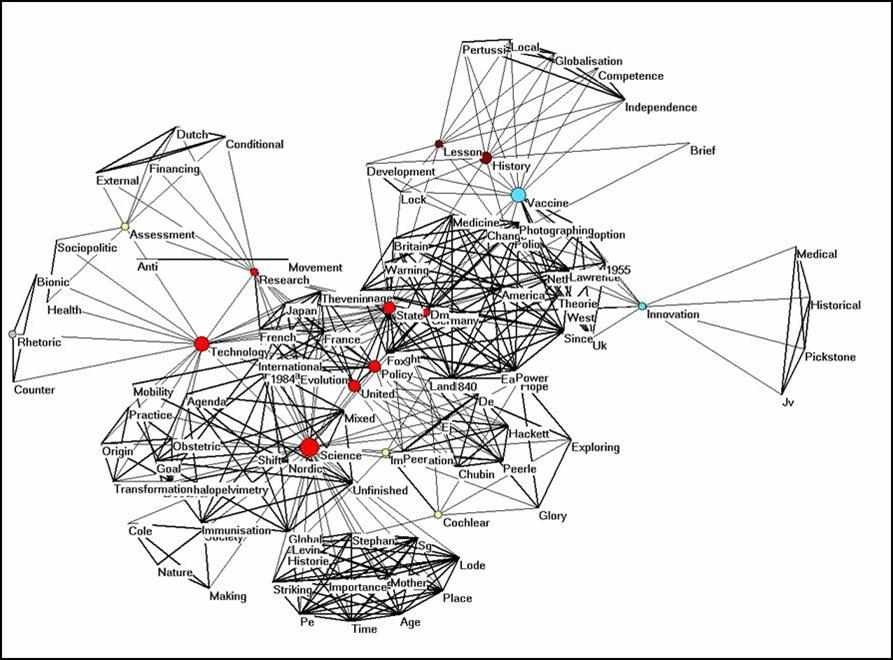
Figure 1: Semantic map for the titles of Stuart Blume contained in the Social Science Citation Index (March 2007).
I removed the unconnected words by partitioning the file (Net > Partition > Core > All) and then Operations > Extract from Network > Partition > 1-*. The unconnected words are in the partition with number zero and thus removed. The lines are set with different width and with size 2, fonts with size 10, and vertices size 8, as defined on the input file. Note that one can edit the input file or edit the partitions under File > Partition > Edit. The program removes the plural s, and you may wish to add this again (either by editing the file cosine.dat using an ASCII editor like NotePad or within Pajek by editing the partitions under File > Partition > Edit).
The program produces more files. You can read the file matrix.dbf into SPSS and then you see that the occurrence matrix contains 22 rows and 104 variables. In SPSS you can compute the cosine matrix by going to Analyze > Correlation > Distance > Between variables > Similarity > Cosine. This procedure is similar to the one done by ti.exe, but SPSS is much faster. In the case of large matrices, this may be an advantage. This file can be analyzed further, for example, using factor analysis or cluster analysis, but this goes beyond the scope of this lesson. These techniques may enable you to legitimate the grouping of words in terms of the statistics. (See the text which you read for today.)
Open the files cosine.dat and coocc.dat using an ASCII editor. Coocc.dat provides the co-word matrix in the so-called DL format of UCINet which can also be read by Pajek. Cosine.dat is in the Pajek format. The parameters x-fact and y-fact determine the size of the nodes in the visualization. There are many more parameters available in Pajek if you wish. The pictures in Pajek can also be exported so that you can use them in Word and other programs. Let’s do this using coocc.dat. Make the picture and save it by using Export > 2D > bmp. Thereafter, import the bmp-file into a Word file using Insert > Picture > From File. In this case the cosine-normalized file is not so different from the co-occurrence picture.
Full text analysis
Let us now rename text.txt text1.txt and copy leydesdorff.txt to text2.txt. Thus, we have two text files and we use the same words.txt file derived from Blume’s title words. Fulltext.exe will generate a matrix of two cases corresponding to the two texts and using the same words as variables (UoA-version). This matrix will be very dense because it has only two rows. If we import the file cosine.dat into Pajek we can generate the following picture, but only after removing the lines with cosine ≤ 0.5. (Net > Transform > Remove > lines with value lower than 0.5). The words which are exclusively used by Blume’s text form now a dense cluster, while the words which the two authors have in common are placed at a distance.
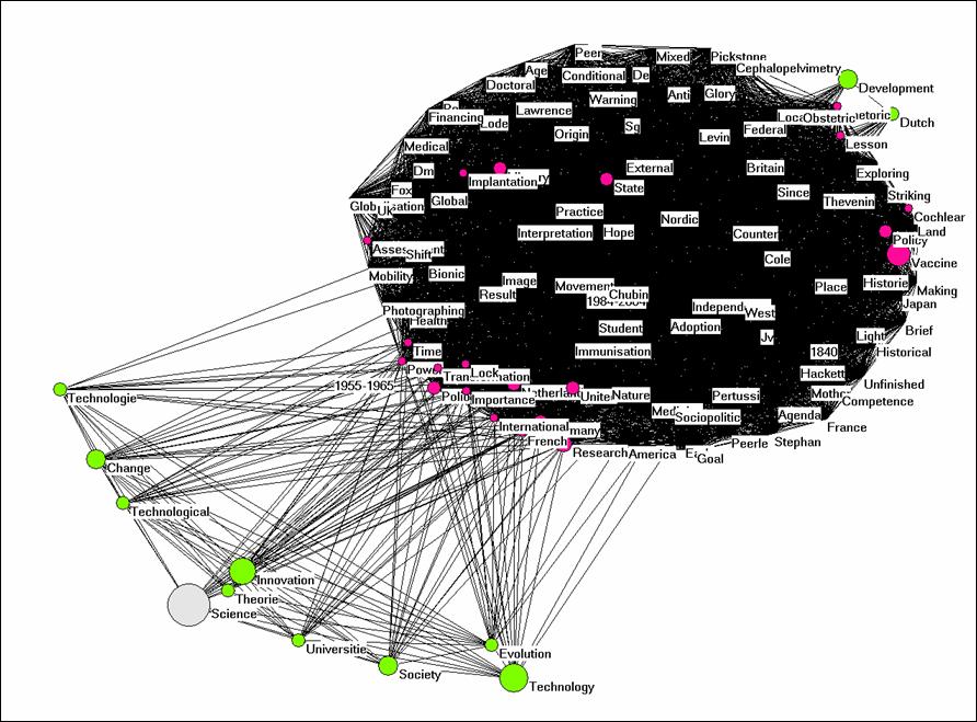
Figure 2: Semantic map of the two texts, cosine ≥ 0.5.
If we now change to the coocc.dat file as input, we have again to select a threshold because otherwise everything is connected with everything. Let’s try the threshold of words occurring five of more times. The Kamada-Kawai solution will provide you with a star-shaped network which bring the most frequently used words to the center. Can you understand why?
It is possible to generated an equivalent to figure 2 using coocc.dat by using Layout > Energy > Fruchterman-Reingold > 2D. Is it an equivalent? It looks like at first sight, but what would count against it.
Exercise
Use one of a few (four or so) of your own texts and do a fulltext-analysis. (Texts have to be saved first as “plain text” using the MS-Dos format and insert CR/LF this time. Texts should after the saving be not larger than 64 kByte. You can rightclick on the text and find out what its size is under “Properties”.)
Embellish the pictures which you can generate from cosine.dat and coocc.dat and write a commentary. What did it teach you about your own writing?
Please read for next week as an introduction Visualization of the Citation Impact Environments of Scientific Journals: An online mapping exercise, Journal of the American Society for Information Science and Technology 58(1), 25-38, 2007 . <pdf-version of the journal from the library>.
Amsterdam, 4 April 2007
References:
Callon, M., Courtial, J.-P., Turner, W. A., & Bauin, S. (1983). From Translations to Problematic Networks: An Introduction to Co-word Analysis,. Social Science Information 22, 191-235.
Callon, M., Law, J., & Rip, A. (Eds.). (1986). Mapping the Dynamics of Science and Technology. London: Macmillan.
Leydesdorff, L. (1997). Why Words and Co-Words Cannot Map the Development of the Sciences. Journal of the American Society for Information Science, 48(5), 418-427.