|
Homepage | Publications | Software; data | Courseware; indicators | Animation | Geo | Search website (Google) |
Mapping the Geography of Science:
Distribution Patterns and Networks of Relations among Cities and Institutes
![]()
(This website is an appendix to Loet Leydesdorff and Olle Persson, “Mapping the Geography of Science: Distribution Patterns and Networks of Relations among Cities and Institutes,” Journal of the American Society for Information Science and Technology 61(8) (2010) 1622-1634; <pdf-version>; <html-version>. If you use this (free) software, it is appreciated if you provide a reference to this source.).
The programs operate on a download of data in the standard (tagged) format at the Web-of-Science interface of the Science Citation Indices[1] and then allow the user to make a geographic mapping of the institutional addresses and their relations using Google Earth, Google Maps, and/or Pajek. An example of an input file—to be used here below—can be found here. This input file then has to be named “data.txt” (DOS text file) and to be stored in the same folder as the programs cities1.exe and cities2.exe. (The various processing steps are summarized in an Appendix at the bottom of this page).
The two programs are to be run sequentially with an intermediate step. (Analogous programs for institutional addresses are inst1.exe and inst2.exe. I will discuss the differences at the end of this file; see the paper for further details.) Cities1.exe is derived from isi.exe and first organizes the data into relational databases. It produces among other things a file named “cities.txt” which contains the city and country information (postcode if available) in standardized format. This file can be opened and then copy-and-pasted into the GPS encoder at http://www.gpsvisualizer.com/geocoder/. Choose the (default) Yahoo! format for the encoding. (Geo-coding can be done automatically using the Sci2 Tool available at https://sci2.cns.iu.edu/user/download.php. However, note that my programs assume the ASCII format of gpsvisualizer for the input; use Ctrl-A and Ctrl-C, Ctrl-V, and save geo.txt as simple ASCII or DOS-file; e.g.: ‘48.202548,16.368805,"Vienna, Austria",-,’). I adapted cities2.exe to the Bing format that is used by this geocoder since Oct. 1, 2013.
Cities1.Exe will prompt the user with three questions: one can set a threshold in terms of a minimal percentage of the total set of city-names in the data or set a minimum number of occurrences. Both these options enable the user to limit the size of the network. The third question enables the user to obtain additionally the cosine-normalized data matrix. This is not advised for large matrices because of adding to the computation time. For large datasets (> 200 nodes) the computation of the co-occurrence matrix may also be time consuming. One then can interrupt the program and use the file “matrix.txt” in Pajek for the construction of the (necessary!) co-occurrence matrix. I’ll explain below how to do this, but let me first focus on the next steps in the main line of the process. (The fourth option in cities1.exe enables the user to turn off the generation of a network; only information about the nodes is provided and cities.txt is generated.)
The output of the geo-coding can be used as input into Cities2.Exe after saving the file as a DOS text file. The program prompts for the name of this file. It produces a number of ouput files in various formats:
1) Cities.kml and cities2.kml can be read into Google Earth and/or uploaded to a website and then be read by Google Maps. These files can also be edited. (kml is a markup language.) Furthermore, kml files can directly be visualized at public websites such as http://display-kml.appspot.com/. Cities.kml contains a standard icon; cities2.kml a smaller and transparent one. In Google Maps, one may prefer cities2.kml;
2) Network.kml contains only the network without the nodes;
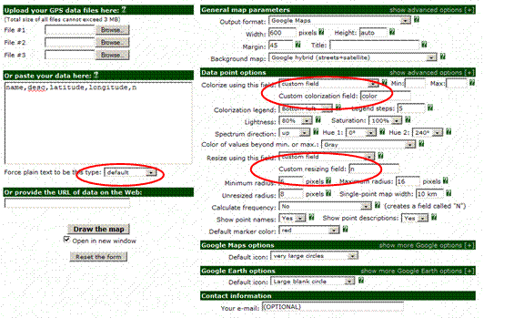
3) Inp_gps.txt can be read into the GPS Visualizer at http://www.gpsvisualizer.com/map_input?form=data. Change the following parameters:
a) Change “waypoints” into “default” underneath the screen input;
b) Change “Colorize using this field” into “custom field”;
c)
Change
“Resize using this field” into “custom field” and “custom resizing field” into
“n”.
The resulting file contains both the nodes and the links. It may take the
browser some time to load it. (If IE gives an error message, try Firefox.)
Networked nodes are (default) in red, not-connected ones in orange. One can
save the file as .html and edit it for usage at one’s own website or locally.
(This file can also be generated within the program BibExcel
using
the additional module at http://www8.umu.se/inforsk/geography/BibExcelGPSexercise.xls.)
|
|
|
|
|
|
4) Cities.paj can be read as a project file into Pajek for network visualization (use <F1> in Pajek); the information in this file can be combined with the file coast.net which contains coastlines based on based on the geographical coordinates of the Coast Line extractor available at the website of the National Geophysical Data Center (NGDC) at http://rimmer.ngdc.noaa.gov/mgg/coast/getcoast.html. We used the World Coast Line data designed to a scale of 1:5,000,000 for this purpose.
The files can be edited and adapted to specific usages. For example, one can change the color of nodes in inp_gps.txt or the color of the network in network.kml. The size of the nodes is set proportionate to the logarithm of its occurrences + 1 (in order to prevent the zero-values of log(1)). The value of the links is equal to the co-occurrence value, but the main diagonal values (co-occurrences within the same city) are not considered. In other words, only the lower triangle of the co-occurrence matrix is used. In the .paj file the links are considered as arcs (but this can be changed into edges).
Further processing in Pajek (ad 4)
Read the .paj file in Pajek (either under File or using <F1> on the keyboard). Read also coast.net into pajek. Pajek allows to keep both networks in a window at the screen and then one can choose under Nets the option Union of vertices. The coastline information is now combined with the network information into a new set. An example of such a complete set can be found here. The network contains now both the address information and the world map. The world map is drawn in term of edges and the network in terms of arcs; these two can therefore be manipulated independently. The full functionality of Pajek (e.g., centrality measures) remains available. Within the Draw screen of Pajek, one can zoom in by drawing a rectangular with a right-mouse click.
Further processing of the html (ad 3)
After drawing the map, click on “save your Google Map”. Use the option to view the source code in your browser and save the source code. Modify the title in line 4, the api-key in line 62, and if so wished, set the zoom to 2 in line 77. Api keys for Google Maps can freely be obtained at http://code.google.com/apis/maps/signup.html. The file will work without an api key at your local computer and with this api key at your website. See for a resulting file at http://www.leydesdorff.net/maps/is2009.html.
A faster way to generate the co-occurrence matrix
Cities1.exe (or inst1.exe) will automatically generate a co-occurrence matrix which is needed in cities2.exe (or inst2.exe, respectively) for the construction of the network. However, this procedure is time-consuming since not based on matrix algebra. (One may wish to run this routine during the night). Alternatively, the program will indicate after a while that one can interrupt using Alt-C. The user is then prompted with the option to discontinue the operation.
At that moment, a file “matrix.txt” is already generated which can be read into Pajek as a network file (File > Read > Network). The co-occurrence matrix can be made in Pajek (v.3) by choosing: Net > 2-Mode Network > Transform > 2-Mode to 1-Mode > Columns. Save the resulting network as a valued matrix with the .mat extension (File > Network > Save). This file should be named “pajek.mat”, and can be read by Paj2Cooc.Exe. This program generates the file coocc.dbf which is needed for cities2.exe or inst2.exe. Note that previous files with the same name are overwritten both by Pajek and by these programs.
Using
the institutional information instead of city names
The programs inst1.exe and inst2.exe work virtually similar to cities1.exe and cities2.exe, but they use the first subfield in the address information in addition to the postal codes, city names, and country names. The first subfield currently contains the organization name (e.g., University of Amsterdam), while the second subfield may contain the name of the sub-organization (e.g., Amsterdam School of Communication Research). However, if the higher-level name lacks, the first field contains the sub-organizational name. Sometimes, the first subfield is a street address (for example, in the case of addresses of corresponding authors).
A further complication arises when organizations use more than a single address. Inst2.exe contains an option not to assemble aggregates of institutional addresses. In that case one answers “N” to the respective question which has “Y” as the default. The network is drawn in both cases on the basis of the same co-occurrence matrix. However, it should work for the nodes.
For an example of the example, see at http://www.leydesdorff.net/maps/institutions.html and http://www.leydesdorff.net/maps/inst.kml (under Google Maps or to be used within Google Earth). These files are constructed for the default option. Without the aggregation: at http://www.leydesdorff.net/maps/inst2.html.
Scopus data
Early 2011, the format of the output of data from Scopus was changed. The previous program scop2isi.exe is therefore no longer reliable. Use instead when downloading data from Scopus, the export facility and choose the following options:
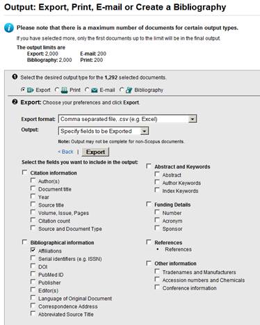
In other words, select only “affiliations” and export in the Excel format to a “comma separated file” which is by default named scopus.csv.
The file “scopus.csv” can be read by scopcity.exe and scopinst.exe which are equivalent to the programs cities1.exe and inst1.exe for data from the Web of Science (SCI, SSCI, A&HCI). Both produce a file called “cities.txt” which can be used for the geocoding as above. One continues with cities2.exe (in both cases).
Note that differently from Web-of-Science data, the post- and zipcodes are needed for the geo-coding of Scopus data because the data is sometimes incomplete. For example, if the indication “United States” is missing, the zip-code containing “MA” is needed for unequivocal identification (as different from Cambridge, UK). However, the post- or zipcodes may lead to fine-graining of the output which is not intended in the case of using cities as units of analysis. Thus, Scopus data can be expected to outperform WoS data for institutional addresses, but not for cities.
If one wishes to prevent this effect, output files of cities2.exe (e.g., inp_gps.txt) have to be edited manually. Another way may be to use the file “data.txt” which is written by scopcity.exe as input to scopcit2.exe which I developed for this purpose. The city addresses in the US and the UK, however, remain difficult to distinguish from their zip-codes or postal codes because the commas were placed irregular in the original Scopus file.
Other data with address information
For other data with address information, one is advised to use the Pajek format and then Paj2Kml.Exe. This is further explained at http://www.leydesdorff.net/gmaps .
Appendix 1: Overview of routines for the data processing.
|
Scopus data ↑ → Scop2Isi.Exe[1] |
Web-of-Science data (in tagged format) |
|
|
|
|
(1) kml-files |
Output
(2) html |
(3) paj-files |
|
|
|
|
|
|
|
|
|
|
|
|
→ |
Cities1.Exe |
→ Cities.txt → |
→ Geo-coding[2] → |
Cities2.Exe |
Cities.kml Cities2.kml |
Inp_gps.txt |
Cities.paj
|
|
|
→ |
Inst1.Exe |
→ Inst.txt |
Inst2.Exe |
Inst.kml |
|
Inst.paj |
|
|
|
|
|
|
|
|
|
|
|
|
|
|
|
↓ |
|
|
↓ |
↓ |
↓ |
|
|
|
|
|
|
|
|
|
|
|
|
|
|
Matrix.txt → |
Possible shortcut to make co-occurrence matrix in Pajek |
|
1. Use with Google Earth |
Input to GPS Visualizer[3] |
Merge with Coast.net[4] within Pajek |
|
|
|
|
|
↓ Paj2Cooc.Exe |
|
2. Upload for Google Maps |
Edit the html (api-key) |
|
|
|
|
|
|
|
|
3. Use at http://display-kml.appspot.com/ |
|
|
Amsterdam, January 2010
[1] For Scopus data, see the special section about Scopus below.
[2] Available at http://www.gpsvisualizer.com/geocoder/ ; geo-coding can be done automatically using the Sci2 Tool available at https://sci2.cns.iu.edu/user/download.php. However, note that my programs assume the format of gpsvisualizer for the input.
[3] Available at http://www.gpsvisualizer.com/map_input?form=data
[4] Available at http://www.leydesdorff.net/maps/coast.zip