1. Introduction
In this communication we report on newly available
methodologies to map the sciences both statically (at each moment of time) and
dynamically (over time). These techniques enable us, among other things, to
visualize patterns of international collaboration using a projection on the
world map (e.g., Glänzel, 2001; Hicks & Katz, 1996; Persson et al.,
2004; Wagner, 2008; Zitt et al., 1999). We compare the different
possibilities in Google Earth, Google Maps, and Pajek, and report on dedicated software
(freeware) available for making these projections using data from bibliographic
databases such as the Science Citation Index and Scopus.
The geographic mapping of science can be distinguished from
its cognitive mapping (Frenken et al., 2009; Jones et al., 2008; Small
& Garfield, 1985). The sciences can be mapped cognitively, for example, in
terms of journal maps (e.g., Leydesdorff, 1986; Tijssen et al., 1987),
co-citations (Small & Griffith, 1974; Small, 1999), or co-words (Callon et
al., 1983). Using techniques such as multi-dimensional scaling (e.g.,
Kruskal & Wish, 1978; Borgatti, 2001; Leydesdorff & Schank, 2008) or
spring-embedded algorithms (e.g., Kamada & Kawai, 1989; Fruchterman & Reingold,
1999), information scientists have made considerable advances during the last
decade in terms of agreeing on similarity criteria (Ahlgren et al.,
2003; Van Eck & Waltman, 2009), possible projections (Boyack et al.,
2005 and 2007; De Moya-Anegón et al., 2007; Klavans & Boyack, 2009a;
Rafols & Leydesdorff, 2009), and even on standard colors for distinguishing
among disciplinary affiliations (Klavans & Boyack, 2009b). The latter
authors suggest that “consensus” has emerged on the mapping. Rafols et al.
(in preparation) drew the conclusion that therefore one would be able to
project developments in science against a statistical baseline.
Since in a socio-cognitive process such as the development
of the sciences, change can take place at different levels at the same time,
Studer & Chubin (1982, at p. 269) already noted that “(r)elationships among
journals, individuals, references, and citations can be analyzed in terms of
their structural properties. But can one be used as a baseline to calibrate our
understanding of another? Does it make sense to attempt to “control” for one
relationship while studying others?” Narin (1976) was the first to distinguish
between nations and disciplines as two analytically independent baselines in
the evaluation (cf. Narin et al., 1972; Narin & Carpenter, 1975).
Small & Garfield (1975) proposed to use these two dimensions as different
bases for the mapping.
Intellectual developments at the global level have also to
be retained locally. National (or regional) governments develop science and
technology policies for this retainment (e.g., Skolnikoff, 1993). Does
investment in science pay off in terms of prominence and reputation, economic
returns, or the emergence of transnational linkages such as envisaged by the
European Commission? (Leydesdorff & Wagner, 2008, 2009; NSB, 2010, pp. 5-33
ff.). Are national governments able to formulate policies which provide them
with a possible hold on “emerging technologies”? Is sufficient knowledge
infrastructure developed to play a role in the case of “generic technologies”?
These and similar questions require a geographic baseline for the assessment in
addition to the cognitive map.
The geographic map, of course, provides us with a natural
baseline for studying the spatial dynamics. In recent years, software
developments have made this map increasingly available for the projection at
different scales and with appropriate zooming techniques, such as in Google
Maps. How can one make such techniques profitable for the enterprise of science
and technology studies? Having both of us been deeply involved in developing
software for using the information contained in databases such as the Science
Citation Index and Scopus for the mapping, we thought it timely to
provide a state-of-the-art review of the current possibilities and limitations
of geographic maps. Where necessary we further developed our software for
bridging gaps and made these tools available from our respective websites. The
interested reader can find instructional materials and manuals at these sites (http://www.leydesdorff.net/maps and http://www8.umu.se/inforsk/bibexcel/,
respectively).
2. Methods and materials
For didactic purposes we shall use a standard set for the various
visualizations. We chose to use the footprint of the field of information
science (IS) in 2009 as available in the address information in the bylines of the
publications. How did we delimit this field? First, Library & Information
Science (LIS) is categorized as a separate subject in the Social Science
Citation Index, but this category covers 61 journals. These lists, however,
are composed for the purpose of information retrieval and therefore not
sufficiently restricted for mapping a specific field (Leydesdorff & Probst,
2009). More restricted lists of IS have been proposed in the literature. Based
on White & McCain (1998, at p. 300), Zhao & Strotman (2008, at p. 2072)
recently provided an updated list of eight journals representing the core of IS,
in their opinion. Using aggregated journal-journal citation data from the Journal
Citation Report 2008, we found 13 journals that contribute more than 1% to
the citations of JASIST and 11 journals that contribute more then 1% to
the citations of Scientometrics. These two sets overlap in eight
journals, of which six are also included in the list of Zhao & Strotman
(2008).
Since we wished to include also the newly added Journal
of Informetrics, we gave priority to our citation-based definition of the
field and included these eight journals in the analysis (Table 1). Using a
search string based on these eight journals, 621 articles could be
retrieved from the Web-of-Science published in the year 2009.
Because we limited the set to articles, however, no records from the Annual
Review of Information Science and Technology—including 10 reviews and one
editorial in 2009—were retrieved. We limited the analysis to this set
(available at http://www.leydesdorff.net/maps/data.zip).
The file includes 1,479 authors at 1,107 institutional addresses.
|
|
Zhao & Strotman (2008)
|
Citation environment JASIST
(2008)
|
Citation environment Scientometrics
(2008)
|
Journals included in this
analysis
|
|
ACM Transations of
Information Systems
|
|
+
|
|
|
|
Annual Review of
Information Science and Technology
|
+
|
+
|
+
|
(+)
|
|
Computation
and Human Behavior
|
|
+
|
|
|
|
Decision Support
Systems
|
|
+
|
|
|
|
Information
Processing & Management
|
+
|
+
|
+
|
+
|
|
Information
Research
|
|
+
|
+
|
+
|
|
Journal of the
American Society for Information Science and Technology
|
+
|
+
|
+
|
+
|
|
Journal of
Documentation
|
+
|
+
|
+
|
+
|
|
Journal of Informetrics
|
|
+
|
+
|
+
|
|
Journal of
Information Science
|
+
|
+
|
+
|
+
|
|
Library &
Information Science Research
|
+
|
+
|
|
|
|
Knowledge Organization
|
|
+
|
|
|
|
Online
Information Review
|
|
|
+
|
|
|
Proceedings of the ASIST
|
+
|
|
|
|
|
Research
Evaluation
|
|
|
+
|
|
|
Research Policy
|
|
|
+
|
|
|
Scientometrics
|
+
|
+
|
+
|
+
|
Table 1: Core journal lists of Information Science
according to Zhao & Strotman (2008); on the basis of the citation impact of
JASIST and Scientometrics in 2008; and our selection of eight
journals in this study.
In a later section, we compare this set with a similar set
downloaded from the Scopus database. This set contained 551 articles
published in 2009 for the same seven journals. The difference (of 70 articles)
finds its origin in the different organization of the database. Scopus
uses publication dates and not tape years: these articles were downloaded on
January 23, 2009.
However, the institutional addresses are differently organized in Scopus.
Since some of our programs carefully parse the address information, we
elaborated a previously existing routine (Scop2ISI.Exe, available at http://www.leydesdorff.net/software/scop2isi)
in order to make the address information in the Scopus data as comparable
with ISI-data as possible. The current version correctly displays most of the
nodes and links on the maps, but the labels may still be incomplete.
The data can be processed using BibExcel (available at www.umu.se/inforsk/bibexcel/) or
ISI.Exe (at http://www.leydesdorff.net/software/isi/index.htm
). The latter routine was further refined for the purpose of this project into
Cities1.Exe (at http://www.leydesdorff.net/maps/index.htm).
We discuss these dedicated extensions below as they become functional to the
argument.
The 1,107 addresses contain 385 unique city names and 593 unique
institutional addresses.
These could be provided with 591 and 697 geo-coordinates, respectively, at http://www.gpsvisualizer.com/geocoder/.
Yahoo! was used for obtaining the coordinates.
With the exception of one institutional address (“Isle Man Int Business Sch,
Douglas 1M2 1QB, UK”), all coordinates could automatically be retrieved.
A co-occurrence matrix among these 392 cities (and 599
institutions, respectively) was the input to the further analysis and mapping. The
city or institutional nodes can be scaled with the respective number of
occurrences (or the logarithm thereof) as will be indicated where appropriate
in the text. The width of the links is set proportionate to the number of
co-occurrence relations. We first develop the argument with the city names
because the institutional addresses generate some further complications (which
will be discussed in a later section).
3. Google Earth and Chaomei Chen’s CiteSpace
The first application that made it possible to generate
geographic maps of science in the Google format was Chaomei Chen’s program CiteSpace.
Chen and colleagues reported about such themes such as “(v)isualizing and
tracking the growth of competing
paradigms” (Chen et al., 2002; cf. Chen, 2003) since
the early 2000s. The program has been elaborated ever since and is publicly
available at http://cluster.ischool.drexel.edu/~cchen/citespace/.
This program requires as input a download of the data in the standard (tagged)
format at the Web-of-Science interface of the Science Citation Indices
and then allows the user to make a geographic mapping of the institutional
addresses and their relations—in addition to the many other facilities for
citation analysis that this program offers.
When one clicks within CiteSpace on the tab
“Geospatial Maps” in the main menu, one can select the option “Google Earth
(KML)” independently of performing a citation analysis of the data. In the
resulting file, links can optionally be included in addition to the nodes. The
program then generates a so-called .kmz file which is the standard input for
Google Earth (Figure 1).
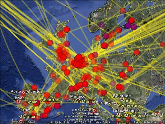
Figure 1: European centers and their network in the
IS set 2009 as output of CiteSpace. (In order to enhance the visibility
when printing in black and white, the color or the network links was changed
from red to yellow.)
Figure 1 provides the result for Europe using our data set.
Within Google Earth, one can zoom in or out and click on links and nodes to
obtain precise address information. In the output file of CiteSpace, the
nodes vary in size as stacked bars which can be seen by tilting the image
horizontally. However, in Google Earth the background is not adjustable from
the satellite image to a street map like under Google Maps and because of the
satellite position in the projection one is not able to draw a global map.
One therefore may wish to bring this information under
Google Maps. Google Maps reads .kmz files when uploaded to a website. It is also
possible to unzip .kmz-files to the .kml format which one can read and edit as a
text file.
(KML is a markup language like HTML.) The resulting kml-file (available at http://www.leydesdorff.net/maps/master-medium.kml)
contains all the information in the map, but this file cannot easily be parsed
and changed, for example, in order to modify the node-sizes in accordance to
the volume of publications. However, one can read this file using the web
address of the upload within Google Maps. Alternatively, there are sites on the
Internet where one can interactively visualize one’s kml-files, such as at http://display-kml.appspot.com/. Using
Google Maps, the problem of different backgrounds can be solved and one is also
able to draw the global map.
4. Google Maps and Google
Earth
The facility to read .kml files into Google Maps provides us
with many options to generate maps from the data by parsing and reformatting
them into this rich markup language. However, the kml-language was primarily
developed for Google Earth. (A subset of kml can also be read by Google Maps
for Mobile.) Thus, the functionality in Google Maps is restricted to only a subset
of tags. For example, one cannot scale the node sizes in Google Maps, but one
can by using the same file in Google Earth. Google Earth, however, does not
allow us to show the global map at a single glance because of the globe format
of the visualization, and has the noted disadvantage of only a single “satellite
view” for the mapping. However, this image can be overlayed with street names
and one can tilt the image.
The various possibilities using a kml-file make this option a
potentially attractive alternative for a number of applications. The
zoom-facilities in Google Maps and Google Earth are superior. Thus, we decided
to further develop this interface. For this purpose, the existing routine ISI.Exe
was further elaborated into Cities1.Exe which can be retrieved from http://www.leydesdorff.net/maps/index.htm.
This program is called Cities1.Exe because after an intermediate step one needs
Cities2.Exe for completing the routine. Cities1.Exe reads the same data as CiteSpace,
but allows users to set relevant thresholds (either in absolute values or as
percentages) on the fly, and to choose for including the generation of a cosine
normalized matrix in addition to a co-occurrence matrix.
The next (and intermediate step) is reading the file
cities.txt—which is one of the outputs of Cities1.Exe—at a geo-coding website
which adds the geographical coordinates to the city names and postcodes. Geo-coding
this information can be done, for example, at http://www.gpsvisualizer.com/geocoder/.
The program Cities2.Exe reads the output of this geocoder and generates, among
other things, the file cities.kml (available at http://www.leydesdorff.net/maps/cities.kml)
which can be uploaded and read by Google Maps or directly into Google Earth.
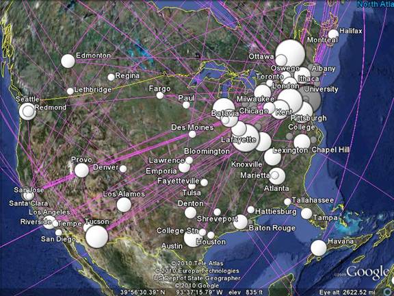
Figure 2: A zoom of cities.kml in Google Earth for
the USA and parts of Canada.
Figure 2 shows the result in Google Earth for the United States. Using the same file in Google Maps (at http://www.leydesdorff.net/maps/cities.kml)
leads to a visually awkward result because the nodes are relatively large and
not scalable. This can be somewhat repaired by using a transparent icon (as at http://www.leydesdorff.net/maps/cities2.kml),
but this change leads unfortunately to a systematic shift in the positioning of
the cities under Google Earth.
However, the resulting picture becomes interesting in Google Maps because both
nodes and links can be visualized, and at variable scales (e.g., globally,
nationally or regionally).
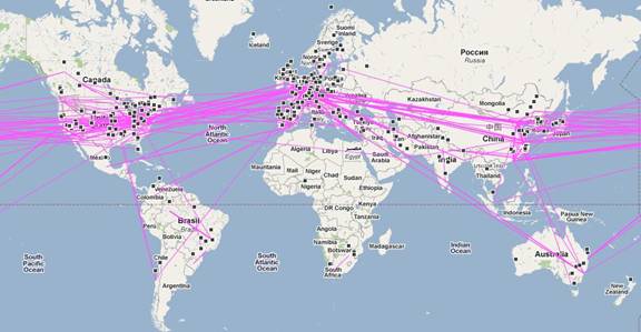
Figure 3: Global map of information science with the
network of coauthorship relations using Google Maps (with http://www.leydesdorff.net/maps/cities2.kml).
Figure 3 shows the global map of IS in 2009 using this
latter option in Google Maps. At the web, the file is clickable and zoomable.
Furthermore, the user can edit the (well-structured) kml file and add
information to the descriptors of nodes and links. One can also adapt the color
of the links. Consequently, this file can be particularly useful for depicting
network dynamics at the web (at various scales). For a dynamic animation one
can collect the output of subsequent representations, for example, in a gif
animator.
In summary, the advantages and disadvantages of using Google
Earth and/or Google Maps are a bit complex, but the kml-file offers a set of
options. Google Maps is particularly useful for the global perspective and for
showing the network dynamics. If the size of the vertices matters and the
perspective is not global but local (or regional), Google Earth provides an
alternative to Google Maps since this program allows for the visualization of
the sizes of the nodes.
5. The GPS Visualizer
As noted, the kml-language is not central to Google Maps
since it was developed for Google Earth. The focus of developers is nowadays on
feeding Google Maps with Javascripts using an API (that is, an application
programming interface). However, this is not easy for the unskilled programmer.
Fortunately, a number of websites come to the rescue of the user. One of them
is the GPS Visualizer at http://www.gpsvisualizer.com/map_input?form=data.
This site allows the user to input data either interactively or to read a file containing
the required input information directly from one’s disk. Cities2.Exe makes this
file available as “inp_gps.txt.” (See for an example, at http://www.leydesdorff.net/maps/inp_gps.txt.)
One can interactively change the various parameters of the
data points on the Google Map to be drawn to the screen. Furthermore, the color
of the nodes can be chosen in the input file (e.g., inp_gps.txt). Cities2.Exe colors
connected nodes red and unconnected ones orange as the default, but one can
edit the file. (Of the 392 nodes used in this study, 97 were not connected in
the network.) Alternatively, BibExcel.Exe contains now a module for generating
this webpage on the basis of ISI data at http://www8.umu.se/inforsk/geography/BibExcelGPSexercise.xls.
The Google Map which is generated at this interface can be
saved both as a picture and in terms of the generating source code (containing
Javascripts). One can adapt this source code within the html. For example, at http://www.leydesdorff.net/maps/IS2009.html,
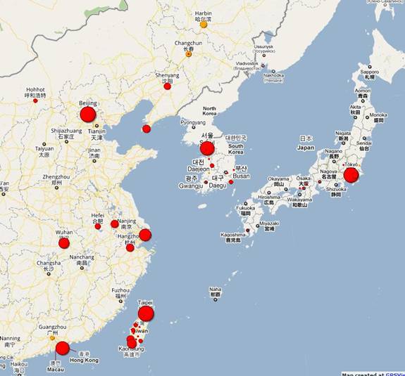
the zoom was reset at “2” instead of “1” for esthetic reasons. (Figure 4
provides a zoom of this file for East Asia.) The resulting files work promptly
at one’s local computer. Before the upload, however, one has to add a “Google
Map API key” at the place which specifies “var
google_api_key = ' ';” within the code. These API keys are freely and
instantaneously available for each web address at http://code.google.com/apis/maps/signup.html.
Figure 4: Visualization of IS in 2009 in East Asia using Google Maps via the GPS Visualizer (at http://www.leydesdorff.net/maps/is2009.html).
In summary, the
use of the GPS Visualizer can have advantages above feeding kml files into
Google Maps. One can vary the sizes and colors of the nodes. Furthermore, one
can make an animation at the web using a so-called redirect statement in the
html (e.g., <meta http-equiv="refresh"
content="5;url=page2.html">). However, the kml files allowed us to
visualize the networks of links in addition to the nodes under Google Maps.
Unfortunately, one cannot have it both ways using these interfaces: one would
like to be able to vary the sizes and colors of both nodes and links. Let us
turn to Pajek as a network visualization program for making this possible.
6. Pajek
In addition
to the kml files and the input for GPS Visualizer, Cities2.Exe also generates a
file “cities.paj” (available at http://www.leydesdorff.net/cities.paj)
which can be read into Pajek as a project file (by using <F1>).
Drawing this file provides a visualization with sizable arcs and vertices. The
vertices are proportionate to the logarithm of the occurrences plus one (since
the log(1) = 0); the links proportionate to the co-occurrences. All statistics
available in Pajek can be applied (De Nooy et al., 2005; Hanneman &
Riddle, 2005). The cities are drawn at their coordinates, and one can directly
compare the geographic map with layouts generated, for example, using the
algorithm of Kamada & Kawai (1989).
A layout in
Pajek can be exported as a transparent overlay using the .eps format. Thus, one
is able to overlay these results on any equirectangular projection of the
worldmap. Additionally, we generated a worldmap in terms of coast lines which
can be imported into Pajek and then merged with the overlay map. This file is available in the Pajek
format at http://www.leydesdorff.net/maps/coast.zip.
If one reads this file into Pajek in addition to cities.paj, one obtains two
networks which can both be selected (in two different Network windows) and then
merged within Pajek using Nets > Union of vertices. One can color and
size the network and the coastlines independently because the latter are
defined in Pajek as edges and the former as arcs.
One can zoom
into Pajek figures by marking a piece of the drawing with a right-clicked
mouse. Using the k-core algorithm in Pajek teaches us, for example, that
the core centers of the coauthorship network in Europe are mostly in Belgium: Antwerp, Louvain, Heverlee—a suburb of Louvain—Oostende, and Diepenbeek. (An additional
relation with Budapest is generated by Wolfgang Glänzel who adds his
affiliation in Budapest routinely to his institutional address in Louvain.) Brussels moreover provides a secondary center with Hamburg, Geneva, Rouen, Paris, and Nantes. This prominent position of Belgium is an artifact of the common
practice of authors in Flanders to publish papers individually at more than a
single city address. We did not correct for this specific effect of the
networking which is induced by policies of the regional government of Flanders (Debackere & Glänzel,
2004).
In a Pajek
drawing of this network, many arcs cross the EU indicating relations between
American and Asian cities. This can be prevented by choosing another projection
of the earth or by refining the set (Figure 5). In the exclusively European network,
most core centers have lost one connection (k = 3 instead of k =
4). In this network, Budapest is no longer part of the core group of Belgian
centers.
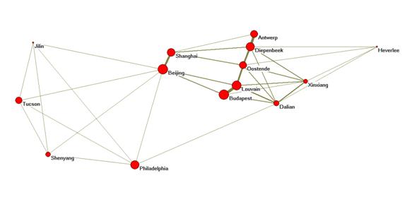
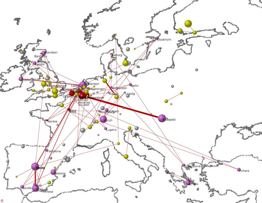
Figure 6:
The network
among 14 core cities in the network of IS 2009 (Kamada & Kawai, 1989).
Figure 6
shows the structure of the (k ≥ 4) core network of the field. The
Belgian groups do not collaborate internationally other than with cities in China and Budapest (Hungary). As noted, these relations among the Belgian (and Hungarian) cities are
largely spurious. The Chinese partners have also American collaborators.
Since one
can package Pajek configurations using the project file format (.paj), the
information can comprehensively be communicated. (One can find the results of
these analyses as examples at http://www.leydesdorff.net/maps/world.zip
and http://www.leydesdorff.net/maps/europe.zip,
respectively.) However, unlike Google Maps the resulting figures cannot be made
interactive at the web. Animations, however, can be made using PajekToSvgAnim, SoNIA or the dynamic version of Visone (Leydesdorff et al., 2008).
7. Institutional collaboration
Strictly
analogous to the programs cities1.exe and cities2.exe, we also developed
inst1.exe and inst2.exe. These latter programs include the first subfields of
the institutional addresses in the ISI data in addition to the city, postcode,
and country information. Using Google Maps, it thus becomes possible to map
relations even at the street level.
The global
map of institutions in the IS 2009 set can be retrieved at http://www.leydesdorff.net/maps/institutions.html.
As before this map contains only the nodes and not the links. Of the 593
institutions, 128 centers were not connected to another one and therefore
colored orange in this map; 557 institution names are unique when one
disregards the different street addresses. At http://www.leydesdorff.net/maps/inst.kml
one finds the file which can be read into Google Maps and Google Earth in order
to show the network relations.
There are a
number of problems because the same institution may publish with different
addresses and addresses are often incomplete. Costas & Irribaren-Maestro
(2007) noted that valuable address information can also be found in the address
of the corresponding author when it fails otherwise in the record. We include
this information in the analysis although it sometimes only contains the postal
address and not the institute’s name.
Institutional
addresses are hierarchically organized in the ISI databases with first the
organization and then the sub-organization (department or faculty) after a
comma as a second subfield. If the name or the organization fails, however, the
sub-organization moves to the first subfield. However, a computer program cannot
evaluate these differences. Thus, we used the first subfield, but always in
combination with the city and country names.
Some
organizations are dispersed over various address (as the Catholic University of
Louvain mentioned above), but in other cases these different addresses host
relatively independent organizations. For example, the Consejo
Superior de Investigaciones Científicas (CSIC) is housed at different
locations in Madrid, but also elsewhere in Spain. In our data, we found 19
records with addresses in Valencia, Sevilla, and Burgassot. In Valencia, however, this same abbreviation (CSIC) is subsumed under the Universita Polytechnica of Valencia.
In summary, the different addresses can be meaningful or
not, and this cannot be decided automatically, but depends on the research
question. The program Inst2.Exe therefore offers the option not to aggregate into
a single institutional name. For most purposes, however, the results of these
fine-grained analyses may contain considerable error. Furthermore, inst2.exe currently
cannot distinguish between different locations of the same institutional name
in terms of the network links. This can be further improved in the future by incorporating
also into inst1.exe the option to disaggregate single institutional names in
terms of different street addresses.
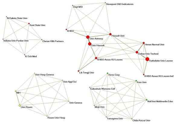
Figure 7: k > 4 networks of collaboration
between leading institutes in the field of information science in 2009.
The (in this
case, aggregated) institutional names provide us with a different view on the
core network among these centers than was above achieved in terms of city
names. Figure 7 shows a highly connected network (k = 6 among 7
partners) of Japanese centers and the Xerox corporation. The figure illustrates
the problem of the various institutional names in the Belgian/Chinese network
at the top (k = 4). The size of the nodes is again proportionate to the
logarithm of the number of papers plus one (in order to prevent a zero as the
evaluation of log(1)). Figure 7 demonstrates the effects of the noted policies
of the Flemish government and the lack of standardization in the naming of
institutions.
8. Scopus
data
The problems
with the institutional identification made us turn to Scopus for the
comparison. Unlike the ISI databases, Scopus is based on index keys and
one might hope that this would make a difference for the standardization. However,
in this database institutional names are even less standardized than in the ISI
data: even delimiters are sometimes missing. Using the 551 articles which could
be retrieved with the equivalent search string, we found, for example, the
three name variants “KU Leuven,” “KULeuven,” and “Katholieke Universiteit
Leuven” among twenty records. As city names, these records
in Scopus contained “Leuven,” “Leuven (Heverlee)”, and “B-3000” that is,
the postcode without mentioning the city. More seriously, two nodes in the
Belgian network (Dalian and Xinxiang) were attributed to addresses in Taiwan according to this database (Liang & Rousseau, 2009). The geo-coder, however,
recognizes this as a mistake and was able to make the correction automatically.
Nevertheless, the city networks using Scopus data are
highly comparable with those based on the ISI set. These files are available at
http://www.leydesdorff.net/maps/scopus.kml
for Google Earth, http://www.leydesdorff.net/maps/scopus2.kml
for Google Maps, http://www.leydesdorff.net/maps/scopus.html
using the GPS Visualizer, and http://www.leydesdorff.net/maps/scopus.paj
for Pajek. The institutional networks suffer from the same problems with
inconsistent naming by authors which hitherto is beyond control for the
database providers, and therefore a fortiori for users without building
extensive thesauri.
9. Conclusions and discussion
We have
wished to show the current possibilities that the bibliometric researcher can
use for the visualization of one’s geographic data, and hopefully provided some
help by developing dedicated software to bridge existing gaps between using on
the one side databases like the Science Citation Index and Scopus
and on the other side the geographical projections in Google Earth, Google Map,
and Pajek. (The various processing steps are summarized in an Appendix.) It
seems to us that for scholarly purposes, the options in Pajek are very rich and
sufficiently beautiful for the illustration. Furthermore, the data in the Pajek
format can be read into a large number of available software programs; for
example, at the Network Bench of Indiana University (at http://nwb.slis.indiana.edu/).
Interfaces with animation programs—for time-series—are also available.
At the
Google interfaces, one can import the complete dataset (as kml or kmz-file)
into Google Earth, but the limitations are inherent to the satellite
projection. Thus, one cannot draw the global map and one has no access to the street
map. The same files can be read into Google Map. In that case, one has the full
scale of projections and the network, but the nodes cannot be scaled. Using GPS
Visualizer, one can scale the nodes, but one looses the network.
Which one of
these options one wishes to use, depends of course on one’s research question. This
contribution was primarily methodological. In addition to network analysis, one
can think, for example, of studies about diffusion and about correlations
between distances and relations (Andersson & Persson, 1993;
Katz, 1994; Wuchty et al., 2007).
Geo-coordinates can be translated into distances using, for example, the
calculator available at www.gpswaypoints.co.za/downloads/distcalc.xls.
The case in
this study was selected so that the results would be recognizable in terms of
flaws by this community. For example, further standardization of the address
information in the bylines seems highly desirable, particularly at the
institutional level. City names are currently sufficiently standardized
(because of postcodes) for research purposes.
The results
further clarify that co-authorship, co-location, collaboration, etc., are all
different dimensions in the scientific enterprise that may or may not overlap
(Katz & Martin, 1997; Wagner, 2008). The relatively new tendency to add
more than a single university address to each author (Persson et al.,
2004) further complicates the issue as we showed for the Belgian case. By
making these tools available, we hope to encourage other information scientists
to be able to use them in a further proliferation of research questions.
Acknowledgement
We are
grateful to Wouter de Nooy and Chaomei Chen for advice and suggestions.
References
Ahlgren, P., Jarneving,
B., & Rousseau, R. (2003). Requirement for a Cocitation Similarity Measure,
with Special Reference to Pearson's Correlation Coefficient. Journal of the
American Society for Information Science and Technology, 54(6), 550-560.
Andersson, Å.,
& Persson, O. (1993). Networking scientists. The Annals of Regional
Science, 27(1), 11-21.
Borgatti, S. P.
(1998). Social Network Analysis Instructional Website, at http://www.analytictech.com/networks/mds.htm.
Boyack,
K. W., Klavans, R., & Börner, K. (2005). Mapping the Backbone of
Science. Scientometrics, 64(3), 351-374.
Boyack,
K., Börner, K., & Klavans, R. (2007). Mapping the Structure and
Evolution of Chemistry Research. Proceedings of the 11th International
Conference of Scientometrics and Informetrics, D. Torres-Salinas & H.
Moed (Eds.), Vol. 1, pp. 112-123, CSIC, Madrid, 21-25 June 2007.
Callon, M.,
Courtial, J.-P., Turner, W. A., & Bauin, S. (1983). From Translations to
Problematic Networks: An Introduction to Co-word Analysis. Social Science
Information 22, 191-235.
Chen, C. (2003). Mapping
Scientific Frontiers: The Quest for Knowledge Visualization. London: Springer.
Chen, C.,
Cribbin, T., Macredie, R., & Morar, S. (2002). Visualizing and tracking the
growth of competing paradigms: Two case studies. Journal of the American
Society for Information Science and Technology, 53(8), 678-689.
Costas,
R., & Iribarren-Maestro, I. (2007). Variations in content and format
of ISI databases in their different versions: The case of the Science Citation
Index in CD-ROM and the Web of Science. Scientometrics, 72(2), 167-183.
De
Moya-Anegón, F., Vargas-Quesada, B., Chinchilla-Rodríguez, Z., Corera-Álvarez,
E., Munoz-Fernández, F. J., & Herrero-Solana, V. (2007). Visualizing
the marrow of science. Journal of the American Society for Information
Science and Technology, 58(14), 2167-2179.
De Nooy, W.,
Mrvar, A., & Batagelj, V. (2005). Exploratory Social Network Analysis
with Pajek. New York: Cambridge University Press.
Debackere, K.,
& Glänzel, W. (2004). Using a bibliometric approach to support research
policy making: The case of the Flemish BOF-key. Scientometrics, 59(2),
253-276.
Frenken, K.,
Hardeman, S., & Hoekman, J. (2009). Spatial scientometrics: towards a cumulative
research program. Journal of Informetrics.
Fruchterman, T.,
& Reingold, E. (1991). Graph drawing by force-directed replacement. Software--Practice
and Experience, 21, 1129-1166.
Glänzel, W.
(2001). National characteristics in international scientific co-authorship
relations. Scientometrics, 51(1), 69-115.
Hanneman, R. A.,
& Riddle, M. (2005). Introduction to social network methods. Riverside, CA: University of California, Riverside; at http://faculty.ucr.edu/~hanneman/nettext/.
Hicks, D., &
Katz, J. S. (1996). Science policy for a highly collaborative science system. Science
and Public Policy, 23(1), 39-44.
Jones, B. F.,
Wuchty, S., & Uzzi, B. (2008). Multi-university research teams: shifting impact,
geography, and stratification in science. Science, 322(5905), 1259-1262.
Kamada, T., &
Kawai, S. (1989). An algorithm for drawing general undirected graphs. Information
Processing Letters, 31(1), 7-15.
Katz, J. S.
(1994). Geographical proximity and scientific collaboration. Scientometrics,
31(1), 31-43.
Katz, J. S.,
& Martin, B. R. (1997). What is research collaboration? Research Policy,
26(1), 1-18.
Klavans, R.,
& Boyack, K. W. (2009a). Identifying Distinctive Competencies in Science. Journal
of Higher Education, under submission.
Klavans, R.,
& Boyack, K. (2009b). Towards a Consensus Map of Science Journal of the
American Society for Information Science and Technology, 60(3), 455-476.
Kruskal, J. B.,
& Wish, M. (1978). Multidimensional Scaling. Beverly Hills, CA: Sage Publications.
Leydesdorff, L.
(1986). The Development of Frames of References. Scientometrics 9,
103-125.
Leydesdorff, L.,
& Schank, T. (2008). Dynamic Animations of Journal Maps: Indicators of
Structural Change and Interdisciplinary Developments. Journal of the
American Society for Information Science and Technology, 59(11), 1810-1818.
Leydesdorff, L.,
& Wagner, C. S. (2008). International collaboration in science and the
formation of a core group. Journal of Informetrics, 2(4), 317-325.
Leydesdorff, L.,
& Wagner, C. S. (2009). Macro-level indicators of the relations between
research funding and research output. Journal of Informetrics, 3(4),
353-362.
Liang, L., &
Rousseau, R. (2009). Bibliometric characteristics of the journal Science:
Pre-Koshland, Koshland and post-Koshland period. Scientometrics, 80(2),
359-372.
Narin, F. (1976).
Evaluative Bibliometrics: The Use of Publication and Citation Analysis in
the Evaluation of Scientific Activity. Washington, DC: National Science
Foundation.
Narin, F.,
Carpenter, M., & Berlt, N. C. (1972). Interrelationships of Scientific
Journals. Journal of the American Society for Information Science, 23,
323-331.
Narin, F., &
Carpenter, M. P. (1975). National Publication and Citation Comparisons,. Journal
of the American Society of Information Science, 26, 80-93.
National Science
Board. (2010). Science and Engineering Indicators. Washington DC: National Science Foundation; available at http://www.nsf.gov/statistics/seind10/.
Persson, O.,
Glänzel, W., & Danell, R. (2004). Inflationary bibliometric values: The
role of scientific collaboration and the need for relative indicators in
evaluative studies. Scientometrics, 60(3), 421-432.
Rafols, I., & Leydesdorff, L. (2009). Content-based and Algorithmic Classifications of
Journals: Perspectives on the Dynamics of Scientific Communication and Indexer
Effects Journal of the American Society for Information Science and
Technology, 60(9), 1823-1835.
Rafols, I., Porter, A., & Leydesdorff, L. (in preparation). Science overlay maps: a new tool
for research policy and library management.
Skolnikoff, E. B.
(1993). The Elusive Transformation: science, technology and the evolution of
international politics. Princeton, NJ: Princeton University Press.
Small, H. (1999).
Visualizing Science by Citation Mapping. Journal of the American Society for
Information Science, 50(9), 799-813.
Small, H., &
Garfield, E. (1985). The geography of science: disciplinary and national
mappings. Journal of Information Science, 11, 147-159.
Small,
H., & Griffith, B. (1974). The Structure of Scientific Literature I. Science
Studies 4, 17-40.
Tijssen,
R., de Leeuw, J., & van Raan, A. F. J. (1987). Quasi-Correspondence
Analysis on Square Scientometric Transaction Matrices. Scientometrics 11,
347-361.
Van
Eck, N. J., & Waltman, L. (2009). How to normalize cooccurrence
data? An analysis of some well-known similarity measures. Journal of the
American Society for Information Science and Technology, 60(8), 1635-1651.
Wagner, C. S.
(2008). The New Invisible College. Washington, DC: Brookings Press.
Wuchty, S.,
Jones, B. F., & Uzzi, B. (2007). The increasing dominance of teams in
production of knowledge. Science, 316(5827), 1036-1039.
Zitt,
M., Barré, R., Sigogneau, A., & Laville, F. (1999). Territorial
concentration and evolution of science and technology activities in the
European Union: a descriptive analysis. Research Policy, 28(5), 545-562.