The semantic mapping of words and co-words in contexts
![]()
Loet Leydesdorff & Kasper Welbers
Amsterdam School of Communication Research (ASCoR), University of Amsterdam
Kloveniersburgwal 48, 1012 CX Amsterdam, The Netherlands
Abstract
Meaning can be generated when information is related at a systemic level. Such a system can be an observer, but also a discourse, for example, operationalized as a set of documents. The measurement of semantics as similarity in patterns (correlations) and latent variables (factor analysis) has been enhanced by computer techniques and the use of statistics; for example, in “Latent Semantic Analysis.” This communication provides an introduction, an example, pointers to relevant software, and summarizes the choices that can be made by the analyst. Visualization (“semantic mapping”) is thus made more accessible.
Keywords: semantic, map, document, text, word, latent, meaning
Introduction
In response to the development of co-citation maps during the 1970s by Small (1973; Small & Griffith, 1974), Callon et al. (1983) proposed developing co-word maps as an alternative to the study of semantic relations in scientific and technology literatures (Callon et al., 1986; Leydesdorff, 1989). Ever since, these techniques for “co-word mapping” have been further developed, for example, into “Latent Semantic Analysis” (e.g., Landauer et al., 1998; Leydesdorff, 1997). These methods operate on a word-document matrix in which the documents can be considered as providing the cases (e.g., rows) to which the words are attributed as variables (columns).
Factor-analytic techniques allow for clustering the words in terms of the documents, or similarly, the documents in terms of the semantic structures of the words (Q-factor analysis). Singular value decomposition combines these two options, but is not so easily available in standard software packages such as SPSS. In this brief communication, we provide an overview and summary for scholars and students who wish to use these techniques as an instrument, for example, in content analysis (Danowski, 2009). A more extensive manual can be found at http://www.leydesdorff.net/indicators where the corresponding software is also made available. In this communication, we provide arguments for choices that were made when developing the software. Our aim is to keep the free software up-to-date, and to keep the applications as versatile and universally applicable as possible.
The word-document matrix
The basic matrix for the analysis represents the occurrences of words in documents. Documents are considered as the units of analysis. These documents can vary in size from large documents to single sentences, such as, for example, document titles. The documents contain words which can be organized into sentences, paragraphs, and sections. The semantic structures in the relations among the words can be very different at these various levels of aggregation (Leydesdorff, 1991, 1995). Thus, the researcher has first to decide what will be considered as relevant units of analysis.
Secondly, which words should be included in the analysis? An obvious candidate for the selection is frequency of word occurrences (after correction for stopwords). Salton & McGill (1983), however, suggested that the most frequently and least frequently occurring words can be less significant than words with a moderate frequency. For this purpose, these authors proposed a measure: the so-called “term frequency-inverse document frequency,” that is, a weight which increases with the frequency of the term i, but decreases as the term occurs in more documents (k) in the set (of n documents). The tf-idf can be formalized as follows:
Tf-Idfik = FREQik * [log2 (n / DOCFREQk)] (1)
The function assigns a high degree of importance to terms occurring more frequently in only a few documents of a collection, and is commonly used in information retrieval (Spark Jones, 1972). Given its background in practice, however, the measure has not been further developed into a statistics for distinguishing the relative significance of terms.
The proper statistics to compare the rows or columns of a matrix is provided by χ2 or—using the Latin alphabet—“chi-square” (e.g., Mogoutov et al., 2008; Van Atteveldt, 2005). Chi-square is defined as follows:
![]() (2)
(2)
The chi-square is summed over the cells of the matrix by comparing for each cell the observed value with the expectation—calculated in terms of the margin totals of the matrix. The resulting sum values can then be tested against a standard table. Both the relevant routines and the chi-square table are now widely available on the Internet; for example, at http://people.ku.edu/~preacher/chisq/chisq.htm. (If the observed values are smaller than five, one should apply the so-called Yates correction; the corresponding statistics is available, for example, at http://www.fon.hum.uva.nl/Service/Statistics/EqualDistribX2.html.)
Our programs—to be discussed below in more detail and available from http://www.leydesdorff.net/indicators—provide the user with the chi-square values for each word as a variable and additionally a file “expected.dbf” which contains the expected values in the same format as the observed values in the file “matrix.dbf.” The user can thus easily compute the chi-square using Excel.[1] Furthermore, the comparison between observed and expected values allows for a third measure which is easy to understand, albeit not based on a statistics, namely, the value of observed over expected (obs/exp). This value can also be compared among aggregates of values over columns which represent variables (words).
In summary, one can use four criteria for selecting the list of words to be included in the analysis: (i) word frequency, (ii) the value of tf-idf, (iii) the contribution of the column to the chi-square of the matrix, and (iv) the margin totals of observed/expected. In case studies, we found this last measure most convenient. However, all four measures can be made available.
The analysis
The asymmetrical word-document matrix—in social network analysis also called a 2-mode matrix—can be transformed into a symmetrical co-occurrence matrix (1-mode) using matrix algebra. This can be done in both (orthogonal) directions, that is, in terms of co-words or co-occurring documents.[2] The resulting matrix is called an affiliations matrix in social network analysis, and is standardly available in software for social network analysis (such as Pajek and UCINet). The resulting network is a relational network.
The word-document matrix can also be analyzed in terms of its latent dimensions using factor analysis, multi-dimensional scaling (MDS) or singular value decomposition (SVD), etc. Note that factor analysis and SVD operate in the vector-space that is generated by first transforming the matrix using the Pearson correlation coefficients between the variables. In the vector space, however, similarity is no longer defined in terms of relations, but correlations among the distributions (vectors).
Since the distributions of words in texts are skewed (Ijiri & Simon, 1977), the use of the Pearson correlation—implying regression to the mean—is debatable (Ahlgren et al., 2003). Salton’s cosine has the advantage of not using the mean, but otherwise its formulation is completely analogous. Cosine-normalization of the variables therefore provides an attractive alternative, but one loses the advantage of orthogonal rotation possible with factor analysis and statistical testing (Bensman, 2003; White, 2003 and 2004). However, one can use the factor-analytic results to color the semantic maps based on cosine-normalized variables (Egghe & Leydesdorff, 2009). Note that it is preferable to factor analyze not the (1-mode) co-occurrence matrix, but the 2-mode word-document matrix if available as a result of the data collection (Leydesdorff & Vaughan, 2006).
In other words, the vector space can be approximated by constructing a semantic map on the basis of cosine-normalized variable patterns or by using factor analysis (or SVD), but these two representations will not be precisely similar. Note that the transition to the vector space changes the perspective from a network perspective (as predominant in social network or co-word analysis) to a systemic perspective. The words are provided with meaning in terms of the semantic structures in the sets, and therefore one can legitimately use concepts such as “latent semantic analysis” and “semantic mapping.”
The results can also be considered as a quantitative form of content analysis (Danowski, 2009; Carley & Kaufer, 1993; Leydesdorff & Hellsten, 2005). Unlike content analysis, however, the semantics is induced from the data and not provided on the basis of an a priori scheme. Thus, one can potentially reduce the so-called “indexer effect” (e.g., Law & Whittaker, 1992).
In summary, the development of statistical techniques has enabled us to move from Osgood et al.’s (1957) initial attempts to measure meaning using 7-point (Likert) scales to automated content analysis which provides us with semantic maps of the intrinsic meaning contained in document sets. Relevant software and techniques for these mapping efforts are available on the Internet.
An empirical example
As an empirical example, we searched the Web-of-Science
(WoS) of Thomson Reuters with the search string ‘ti= “impact factor” and py = (2008
or 2009)’ on November 12, 2010. This search resulted in 195 documents; these
documents contain 59 words which occur more than twice (after correction for
stop words; for example, at http://www.lextek.com/manuals/onix/stopwords1.html).
Using the routine “ti.exe”—available at http://www.leydesdorff.net/software/ti/index.htm—one
can perform factor analysis of the matrix and/or normalize the column variables
using the cosine for the visualization. In Figure 1, the rotated factor matrix
was used to colour the nodes in the map based on the cosine-normalized word
occurrences over the documents.
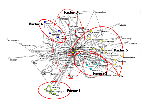
Figure 1: Five factors in 59 words as variables occurring more than
twice in 195 documents with “impact factor” in the title and published in 2008
or 2009 (Kamada & Kawai, 1989; Factor loadings and cosine values < 0.1
are suppressed).
The results as shown in Figure 1 are not completely satisfactory; words which load on Factor 3 are displayed on both sides of the search terms “Impact” and “Factor”. By changing to the observed/expected ratios, Figure 2 can be generated analogously. The word “Factor” in this case no longer loads positively on any of the five factors, but exhibits interfactorial complexity. However, the (different!) factor structure can in this case be penciled contingently on top of this semantic map. Note that many words do not exhibit factor loadings on any of the factors above the level of 0.1 (and are therefore left white).
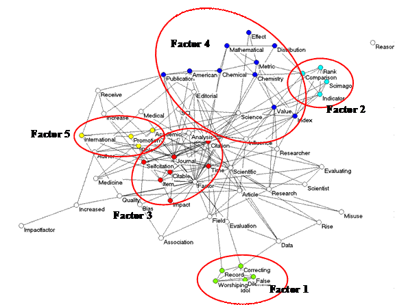
Figure 2: Five factors as in Figure 1, but now with observed/expected
values as input instead of observed values.
In the above figures, only positive factor loadings were used for the coloring. Another visualization which includes also negative factor loadings can be generated by feeding the rotated component matrix directly into the visualization program as an asymmetrical (2-mode) matrix. This leads in this case to Figure 3. The factor loadings are by definition equal to the Pearson correlation coefficients among the variables (vectors) and latent dimensions (eigenvectors). The two constructs—vectors and eigenvectors—can thus be projected onto a single vector space (Leydesdorff & Probst, 2009).
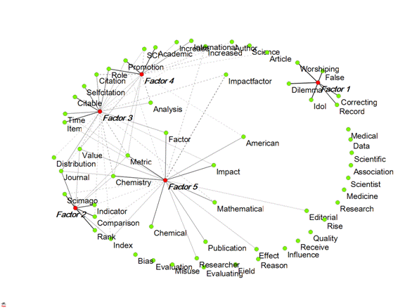
Figure 3: Visualization of the rotated factor matrix; dotted lines
represent negative factor loadings (Fruchterman & Reingold, 1991). Factor
loadings between -0.1 and +0.1 were suppressed.
One possible advantage of this representation is facilitation of the factor designation. For example, Factor 1 is otherwise isolated and indicates a set of words (a “frame”; cf. Hellsten et al., 2010; Scheufele, 1999) critical to the use of impact factors in research evaluation. Factor 5 seems most connected to the other three groupings; it shows the conceptual origins of “impact factor.” This Factor 5 is most interrelated to Factor 3 which provides the frame of “citation analysis.” The words “Factor,” “Value,” and “Metric” provide articulation points between these two star-shaped graphs. “Value” and “Metric” also relate to Factor 2, which indicates more recent ranking efforts.
Figures for different years can also be animated using a version of the network program Visone specially designed for this purpose (at http://www.leydesdorff.net/visone; Leydesdorff & Schank, 2008). In addition to statistical packages, the various output files (in the Pajek format) can also be imported into other network programs such as VosViewer available at http://www.vosviewer.org (Van Eck & Waltman, 2010) or the Social Networks Image Animator (SoNIA) at http://www.stanford.edu/group/sonia/ (Bender-de Moll & McFarland, 2006; Moody et al., 2005).
Conclusions and summary
Despite the emphasis in the wording on semantics (as in “latent semantic analysis,” “the semantic web” or “semantic mapping”), the measurement of the dynamics of meaning is still in its infancy. Meaning is generated when different bits of information are related at the systems level, and thus positioned in a vector space. Perhaps, one can define “knowledge” recursively as the positioning of different meanings in relation to one another.
Note that in the above, semantics is considered as a property of language, whereas meaning is often defined in terms of use (Wittgenstein, 1953), that is, at the level of agency. Ever since the exploration of intersubjective “meaning” in different philosophies (e.g., Husserl, 1929; Mead, 1932), the focus in the measurement of meaning has gradually shifted to the intrinsic meaning of textual elements in discourses and texts, that is, to a more objective and supra-individual level. The pragmatic aspects of meaning can be measured using Osgood et al.’s (1957) Likert-scales and by asking respondents. Modeling the dynamics of meaning requires another elaboration (cf. Leydesdorff, 2010).
References:
Ahlgren, P., Jarneving, B., & Rousseau, R. (2003). Requirement for a Cocitation Similarity Measure, with Special Reference to Pearson’s Correlation Coefficient. Journal of the American Society for Information Science and Technology, 54(6), 550-560.
Bender-deMoll, S., & McFarland, D. A. (2006). The art and science of dynamic network visualization. Journal of Social Structure, 7(2), http://www.cmu.edu/joss/content/articles/volume7/deMollMcFarland/.
Bensman, S. J. (2004). Pearson’s r and Author Cocitation Analysis: A Commentary on the Controversy. Journal of the American Society for Information Science and Technology, 55(10), 935-936.
Callon, M., Courtial, J.-P., Turner, W. A., & Bauin, S. (1983). From Translations to Problematic Networks: An Introduction to Co-word Analysis. Social Science Information 22(2), 191-235.
Callon, M., Law, J., & Rip, A. (Eds.). (1986). Mapping the Dynamics of Science and Technology. London: Macmillan.
Carley, K. M., & Kaufer, D. S. (1993). Semantic connectivity: An approach for analyzing symbols in semantic networks. Communication Theory, 3(3), 183-213.
Danowski, J. A. (2009). Inferences from word networks in messages. In K. Krippendorff & M. A. Bock (Eds.), The content analysis reader (pp. 421-429). Los Angeles, etc.: Sage.
Fruchterman, T., & Reingold, E. (1991). Graph drawing by force-directed replacement. Software--Practice and Experience, 21, 1129-1166.
Hellsten, I., Dawson, J., & Leydesdorff, L. (2010). Implicit media frames: Automated analysis of public debate on artificial sweeteners. Public Understanding of Science, 19(5), 590-608.
Husserl, E. (1929). Cartesianische Meditationen und Pariser Vorträge [Cartesian meditations and the Paris lectures]. The Hague: Martinus Nijhoff, 1973.
Ijiri, Y., & Simon, H. A. (1977). Skew Distributions and the Sizes of Business Firms Amsterdam, etc.: North Holland).
Kamada, T., & Kawai, S. (1989). An algorithm for drawing general undirected graphs. Information Processing Letters, 31(1), 7-15.
Landauer, T. K., Foltz, P. W., & Laham, D. (1998). An introduction to latent semantic analysis. Discourse processes, 25(2), 259-284.
Law, J., & Whittaker, J. (1992). Mapping acidification research: A test of the co-word method. Scientometrics, 23(3), 417-461.
Leydesdorff, L. (1989). Words and Co-Words as Indicators of Intellectual Organization. Research Policy, 18(4), 209-223.
Leydesdorff, L. (1991). In Search of Epistemic Networks. Social Studies of Science, 21, 75-110.
Leydesdorff, L. (1995). The Challenge of Scientometrics: The development, measurement, and self-organization of scientific communications. Leiden: DSWO Press, Leiden University; at http://www.universal-publishers.com/book.php?method=ISBN&book=1581126816.
Leydesdorff, L. (1997). Why Words and Co-Words Cannot Map the Development of the Sciences. Journal of the American Society for Information Science, 48(5), 418-427.
Leydesdorff, L. (2010). The Communication of Meaning and the Structuration of Expectations: Giddens’ “Structuration Theory” and Luhmann’s “Self-Organization”. Journal of the American Society for Information Science and Technology, 61(10), 2138-2150.
Leydesdorff, L., & Hellsten, I. (2005). Metaphors and Diaphors in Science Communication: Mapping the Case of ‘Stem-Cell Research’. Science Communication, 27(1), 64-99.
Leydesdorff, L., & Probst, C. (2009). The Delineation of an Interdisciplinary Specialty in terms of a Journal Set: The Case of Communication Studies. Journal of the American Society for Information Science and Technology, 60(8), 1709-1718.
Leydesdorff, L., & Vaughan, L. (2006). Co-occurrence Matrices and their Applications in Information Science: Extending ACA to the Web Environment. Journal of the American Society for Information Science and Technology, 57(12), 1616-1628.
Mead, G. H. (1934). The Point of View of Social Behaviourism. In C. H. Morris (Ed.), Mind, Self, & Society from the Standpoint of a Social Behaviourist. Works of G. H. Mead (Vol. 1, pp. 1-41). Chicago and London: University of Chicago Press.
Mogoutov, A., Cambrosio, A., Keating, P., & Mustar, P. (2008). Biomedical innovation at the laboratory, clinical and commercial interface: A new method for mapping research projects, publications and patents in the field of microarrays. Journal of Informetrics, 2(4), 341-353.
Moody, J., McFarland, D., & Bender-deMoll, S. (2005). Dynamic Network Visualization. American Journal of Sociology, 110(4), 1206-1241.
Osgood, C. E., Suci, G., & Tannenbaum, P. (1957). The measurement of meaning. Urbana: University of Illinois Press.
Salton, G., & McGill, M. J. (1983). Introduction to Modern Information Retrieval. Auckland, etc.: McGraw-Hill.
Scheufele, D. A. (1999). Framing as a theory of media effects. The Journal of Communication, 49(1), 103-122.
Small, H. (1973). Co-citation in the Scientific Literature: A New measure of the Relationship between Two Documents. Journal of the American Society for Information Science, 24(4), 265-269.
Small, H., & Griffith, B. (1974). The Structure of Scientific Literature I. Science Studies 4, 17-40.
Spark Jones, K. (1972). A statistical interpretation of term importance in automatic indexing. Journal of Documentation, 28(1), 11-21.
Van Atteveldt, W. (2005). Automatic codebook acquisition. Paper presented at the workhop Methods and Techniques Innovations and Applications in Political Science Politicologenetmaal 2005 Antwerp, 19-20 May 2005; available at http://www.vanatteveldt.com/pub/pe05WvA.pdf.
Van Eck, N. J., & Waltman, L. (2010). Software survey: VOSviewer, a computer program for bibliometric mapping. Scientometrics, 84(2), 523-538.
White, H. D. (2003). Author Cocitation Analysis and Pearson’s r. Journal of the American Society for Information Science and Technology, 54(13), 1250-1259.
White, H. D. (2004). Reply to Bensman. Journal of the American Society for Information Science and Technology, 55(9), 843-844.
Wittgenstein, L. (1953). Philosophical investigations. New York: Macmillan.